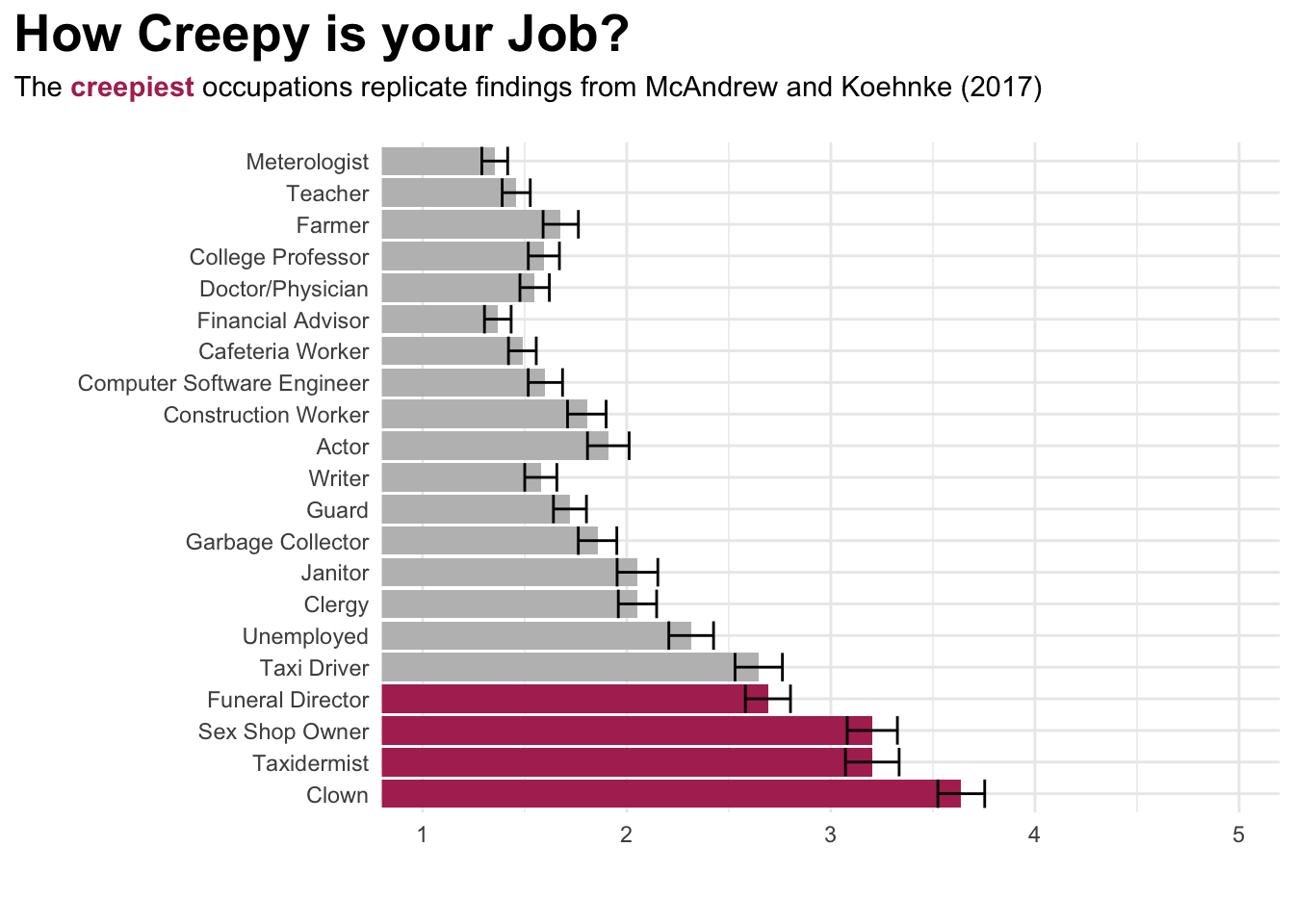
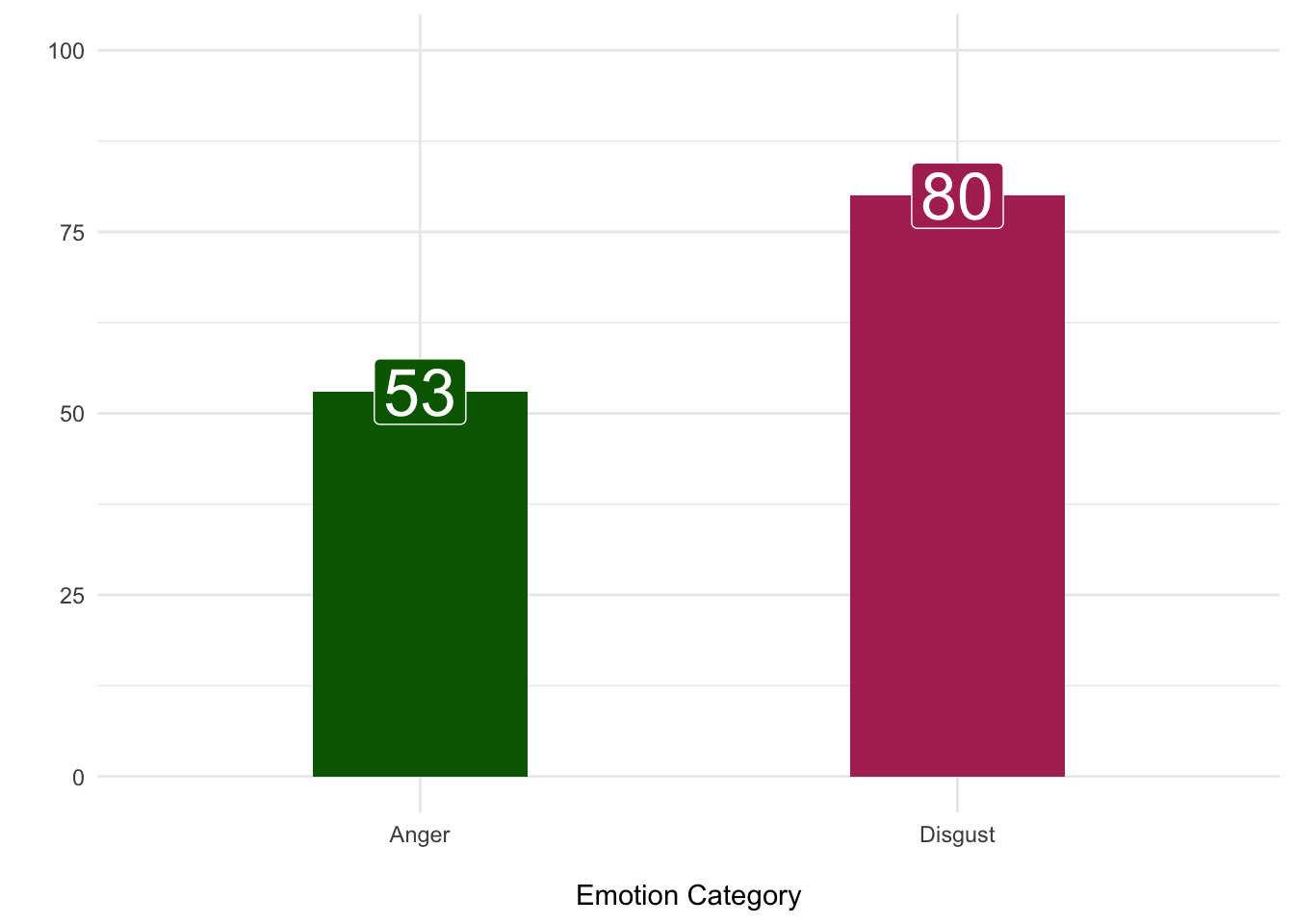
Perceptions of Creepiness

Hypotheses

Stimuli

Data Processing

# Load in packages
library(haven) # Import SPSS
library(dplyr) # Wrangling Data
library(tibble) # Nicer Printing
library(tidyr)  #  Manipulate Data
library(ggplot2) # Plotting Data
library(purrr) # Dealing with lists
library(labelled) #  For dealing with labels
library(forcats) # for handling categories
library(huxtable)  # For making nice tables
library(afex) # for nice ANOVAS
library(broom) # Cleaning up stats
library(stringr) # Text Manipulation
library(janitor) # Cleaning up names
library(tidytext) # Word Count
library(patchwork) # Combining Graphs
library(readxl) # Read in excel
library(ggtext) # Add text elements to plots
suppressPackageStartupMessages(library(googleVis))

# Custom Functions 
discrete_tab <- function(data,x){
  name <- 
    data |> 
    select({{x}}) |> 
    pull()

  tab <- 
    name |> 
    tabyl() |> 
    select(-(starts_with("val"))) |> 
    # Ignore Error for Now,,,
    adorn_pct_formatting(,,,percent) |> 
    rename_with(str_to_sentence) |> 
    hux() |> 
    theme_article() |> 
    set_align(everywhere,everywhere,".")
  
  tab[1,] <- c(str_to_sentence(x),"","")
  
  tab
}


clean_up <- function(string) {
  string <- str_trim(string)
  string <- str_remove_all(string, "[[:punct:]]")
}


# Read Data
cr <- read_spss("Perceptions+of+Creepiness_February+19%2C+2024_16.43.sav")

# Clean Data
cr_cln <- 
  cr |> 
  # Only look at complete cases
  filter(Finished == 1) |> 
  # Only use 18+ cases
  filter(Age > 1) |> 
  # Remove uneeded columns 
  select(!StartDate:RecordedDate) |> 
  select(!DistributionChannel:UserLanguage) |> 
  select(!id:Ethnicity_Race_6_TEXT___Topics) |> 
  rename(
    Creepy_Occ_8 = Occ_8)

Demographics

# Subset Demographic data
demo <- 
  cr_cln |> 
  select(Gender,Religion,Ethnicity_Race,Age) |> 
  mutate(
    # Get Labels of Demographic variables
    Gender = sjlabelled::get_labels(cr_cln$Gender)[cr_cln$Gender],
    Religion = sjlabelled::get_labels(cr_cln$Religion)[cr_cln$Religion],
    Ethnicity_Race = sjlabelled::get_labels(cr_cln$Ethnicity_Race)[cr_cln$Ethnicity_Race],
    Age = sjlabelled::get_labels(cr_cln$Age)[cr_cln$Age])

# Apply Custom Function
gen <- discrete_tab(demo,"Gender")

eth <- discrete_tab(demo,"Ethnicity_Race")

rel <- discrete_tab(demo,"Religion")

age <- discrete_tab(demo,"Age")

gen |> 
  add_rows(eth) |> 
  add_rows(rel) |> 
  add_rows(age) |> 
  # Add Header Row
  insert_row("Variable","N","Percent") |> 
  set_top_border(row = 1:3,1:3) |> 
  set_align(col = 1, value = "left") |>  
  set_align(1,1,"center") |> 
  set_bottom_border(row = nrow(all), col = ncol(all), value = .4) 

Variable	N	Percent
Gender
Female	101	75.9%
Male	29	21.8%
Other	1	0.8%
	2	1.5%
Ethnicity_race
American Indian or Alaska Native	1	0.8%
Asian	20	15.0%
Black or African American	21	15.8%
Other	24	18.0%
White	67	50.4%
Religion
Buddhism	1	0.8%
Christianity	74	55.6%
Islam	16	12.0%
Judaism	2	1.5%
None (atheism)	24	18.0%
Other	16	12.0%
Age
18 - 24	108	81.2%
25 - 34	15	11.3%
35 - 44	3	2.3%
45 - 54	6	4.5%
55 - 64	1	0.8%

Creepy Occupations

Participants were asked to rate 21 occupations on a scale from 1 (Not Creepy at all) to 5 (Very Creepy)

# Get Occupation Labels
occ_lab <- 
  cr_cln |> 
  select(contains("Occ")) 

occ_val <- map_df(occ_lab,get_label_attribute)

# Isolated Occupations
occ <- 
  occ_val |> 
  pivot_longer(cols=Creepy_Occ_2:Creepy_Occ_22,
               names_to = "occ") |> 
  select(value)

# Occupation Analysis
occ <- 
  cr_cln |> 
  rename_at(vars(contains("occ")), ~ occ$value) |>
  pivot_longer(cols = Clown:Meterologist,
               names_to = "jobs",
               values_to = "score") |> 
  mutate(jobs = as.factor(jobs),
         color = ifelse(jobs %in% c("Funeral Director",
                                    "Sex Shop Owner",
                                    "Taxidermist",
                                    "Clown"),"maroon","grey")) 

# Visualize
occ |> 
  ggplot(aes(score,fct_inorder(jobs))) +
  stat_summary(
    fun = "mean",
    geom = "bar",
    aes(fill = color)
  ) +
  stat_summary(
    fun.data = "mean_se",
    geom = "errorbar"
  ) +
  theme_minimal() +
  labs(
    x = "\n",
    y = "\n",
    title = "How Creepy is your Job?",
    subtitle = "The <strong><span style = 'color:maroon;'>creepiest</span></strong> occupations replicate findings from McAndrew and Koehnke (2017)<br>"
  ) +
  coord_cartesian(xlim=c(1,5)) +
  scale_fill_identity() +
  theme(
    plot.title.position = "plot",
    plot.title = element_text(face = "bold",
                              size = 20),
    plot.subtitle = element_markdown()
  )

occ |> 
  group_by(jobs) |> 
  summarize(
    Mean = mean(score),
    SD = sd(score)
  ) |> 
  arrange(desc(Mean)) |> 
  rename(Occupation = jobs) |> 
  hux() |> 
  theme_article()

Occupation	Mean	SD
Clown	3.64	1.32
Sex Shop Owner	3.2	1.42
Taxidermist	3.2	1.52
Funeral Director	2.69	1.27
Taxi Driver	2.65	1.34
Unemployed	2.32	1.26
Clergy	2.05	1.08
Janitor	2.05	1.15
Actor	1.91	1.18
Garbage Collector	1.86	1.09
Construction Worker	1.8	1.09
Guard	1.72	0.932
Farmer	1.68	0.997
Computer Software Engineer	1.6	0.969
College Professor	1.59	0.879
Writer	1.58	0.906
Doctor/Physician	1.55	0.83
Cafeteria Worker	1.49	0.784
Teacher	1.46	0.793
Financial Advisor	1.37	0.754
Meterologist	1.35	0.73

Emotional Perception

Participants were shown two faces from the MSFDE database that either displayed Anger or Disgust. They were then asked to choose the emotion that expresses how they feel toward a supposed Creepy person.

# 1 = Anger | 2 = Disgust
cr_emot <- 
  cr_cln |> 
  select(Emotion) |> 
  remove_labels() |> 
  mutate(
    category = ifelse(Emotion == "1", "Anger","Disgust")
  )

# Chi Square Test Shows More Endorsement for Disgust
table(cr_emot$category) |> 
  chisq.test() |> 
  tidy() |> 
  rename(
    chi = statistic,
    df = parameter,
    p = p.value
  ) |> 
  select(-method) |> 
  select(chi,df,p) |> 
  hux() |> 
  theme_article()

chi	df	p
5.48	1	0.0192

Emotion Visualized

cr_emot |> 
  group_by(category) |> 
  count() |> 
  ggplot(aes(category,n,fill = category, label = n)) + 
  geom_bar(stat = "identity",
           width = .40) +
  theme_minimal() +
  geom_label(size = 9,
             colour = "white") +
  labs(
    x = "\nEmotion Category",
    y = ""
  ) +
  ylim(0,100)+
  theme(
    legend.position = "none"
  ) +
  scale_fill_manual(values = c("darkgreen","maroon"))

Moral Perception

Participants were shown three questions relating to character judgments of a supposed Creepy individual. The three questions were averaged to create a composite score of moral character, with higher values suggesting bad moral character.

mc <- 
  cr_cln |> 
  remove_labels()

# One Sample T-Test showing Creepy People are thought to possess 'bad' moral character
mc |> 
  rowwise() |> 
  select(bad_or_good:trustworthy_r) |> 
  mutate(
    character = mean(c_across(bad_or_good:trustworthy_r))
  ) |> 
  select(character) |> 
  ungroup() |> 
  t.test(mu = 4) |> 
  tidy() |> 
  rename(
    Mean = estimate,
    t = statistic, 
    p = p.value,
    df = parameter
  ) |> 
  mutate(
    `CI[ll,uu]` = paste0("[",
                         conf.low |> round(0),
                         ",",conf.high |> round(0),
                         "]")
  ) |> 
  select(-conf.low,-conf.high,-method,-alternative) |> 
  relocate(p, .after = last_col()) |> 
  hux() |> 
  theme_article() |> 
  set_align("center")

Mean	t	df	CI[ll,uu]	p
6.36	16.8	132	[6,7]	1.42e-34

Face Ratings

pics <- 
  cr_cln |> 
  select(matches("M\\d+_\\d")) |> 
  pivot_longer(
    cols = matches("M\\d+_\\d"),
    values_to = "ratings"
  ) |> 
  mutate(
    attribute = 
      case_when(
        str_detect(name,"M\\d+_1") ~ "Attractiveness",
        str_detect(name,"M\\d+_2") ~ "Trustworthiness",
        str_detect(name,"M\\d+_3") ~ "Dominance",
        str_detect(name,"M\\d+_4") ~ "Creepiness"
    )
  ) 

# Pictures Ranked by Average Rating
pics_avg <- 
  pics |> 
  group_by(name,attribute) |> 
  summarize(
    Mean = mean(ratings,na.rm = TRUE),
    SD = sd(ratings,na.rm = TRUE)
  ) |> 
  arrange(Mean)

`summarise()` has grouped output by 'name'. You can override using the
`.groups` argument.

# Correlations
at <- 
  pics_avg |> 
  filter(attribute == "Attractiveness")

tr <- 
  pics_avg |> 
  filter(attribute == "Trustworthiness")

crp <- 
  pics_avg |> 
  filter(attribute == "Creepiness")

# Attractive x Trustworthiness
cor.test(at$Mean,tr$Mean)

    Pearson's product-moment correlation

data:  at$Mean and tr$Mean
t = 34.674, df = 38, p-value < 2.2e-16
alternative hypothesis: true correlation is not equal to 0
95 percent confidence interval:
 0.9707956 0.9918657
sample estimates:
      cor 
0.9845618 

cor.test(tr$Mean,crp$Mean)

    Pearson's product-moment correlation

data:  tr$Mean and crp$Mean
t = 18.444, df = 38, p-value < 2.2e-16
alternative hypothesis: true correlation is not equal to 0
95 percent confidence interval:
 0.9040064 0.9725928
sample estimates:
      cor 
0.9484314 

cor.test(at$Mean,crp$Mean)

    Pearson's product-moment correlation

data:  at$Mean and crp$Mean
t = 17.872, df = 38, p-value < 2.2e-16
alternative hypothesis: true correlation is not equal to 0
95 percent confidence interval:
 0.8984055 0.9709326
sample estimates:
      cor 
0.9453481 

Qualitative Analyses

Creepiness Scenario

scen <- 
  cr_cln |> 
  select(Creepiness_Scenario) |> 
  filter(!str_detect(Creepiness_Scenario,"test|TEST")) |> 
  separate_longer_delim(
    cols = Creepiness_Scenario,delim = c(",")) |> 
  separate_longer_delim(
    cols = Creepiness_Scenario,delim = c("and")) |> 
  separate_longer_delim(
    cols = Creepiness_Scenario,delim = c(";")) |> 
  mutate(
    Creepiness_Scenario = str_trim(Creepiness_Scenario,"left"),
    Creepiness_Scenario = str_to_lower(Creepiness_Scenario),
    length = str_length(Creepiness_Scenario),
    speaker = row_number()
  ) |> 
  filter(str_detect(Creepiness_Scenario,"^\\b")) |> 
  filter(length > 10) |> 
  slice_sample(n = 20)


gvisWordTree(
    scen,
    chartid = "scenario",
    textvar = "Creepiness_Scenario",
    options=list(width=2000, 
                 height=1000)) |> 
  plot(tag = NULL)

starting httpd help server ... done

Creepy Hobbies

hob <- 
  cr_cln |> 
  select(Creepy_Hobby) |> 
  # Remove single answer and placeholder text
  filter(!str_detect(Creepy_Hobby,"^h|(s){3}\\1")) |> 
  # Separate by (, and or)
  separate_longer_delim(
    cols = Creepy_Hobby,delim = c(",")) |> 
  separate_longer_delim(
    cols = Creepy_Hobby,delim = c("and")) |> 
  mutate(
    Creepy_Hobby = str_trim(Creepy_Hobby,"left"),
    Creepy_Hobby = str_to_lower(Creepy_Hobby)
  )

creep_gv <- 
  gvisWordTree(data = hob, 
             textvar = "Creepy_Hobby",
             chartid = "hobby",
             options=list(width=2000, 
                 height=1000))