Effective and Ineffective Traits in College Instructors as Ranked by College Students
Authors
Affiliations
David Brocker
Farmingdale State College
Vicki Pizanis
Educators Platform
Maggie Rivera
Farmingdale State College
Annette Smith
Dallas College
Tanya Villalpando
University of Missouri - Kansas City
Data Processing
Data was cleaned by renaming all variables to adopt the same naming structure (no spaces, no punctuation, etc.). Next, all identifiers were removed from the dataset. Variables containing metadata were removed as they were not vital to the analyses (Start Date, End Date, Duration, etc.).
After the data was cleaned, trait names were extracted from the column names using regular expressions and the columns were then renamed.
Code
# Load in packageslibrary(haven)library(labelled)library(tidyverse)library(janitor)library(huxtable)library(broom)library(ggplot2)library(skimr)library(purrr)library(stringr)library(forcats)library(patchwork)library(ggtext)library(tidytext)library(wordcloud2)library(irr)library(forcats)library(hrbrthemes)library(sysfonts)library(Rfast)# Custom Functionsdiscrete_tab <-function(data,x){ name <- data |>select({{x}}) |>pull() tab <- name |>tabyl(show_NA =FALSE, show_missing_levels =FALSE) |># Ignore Error for Now...adorn_pct_formatting(,,,percent) |>rename_with(str_to_sentence) |>hux() |>theme_article() |>set_align(everywhere,everywhere,".") |>set_na_string("NA") tab[1,] <-c(str_to_sentence(x),"N","%","Valid %") tab}# Load dataet <-read_sav("Dental+Hygiene+Student+Perceptions+of+Effective+and+Ineffective+Clinical+Teaching+and+Instruction_April+2,+2024_12.43.sav")# Clean Dataet_cln <- et |># Clean Namesclean_names() |># Only Look at Complete Casesfilter(finished ==1) |># Remove identifiersselect(-consent_form) |># Select needed columnsselect(!start_date:recorded_date) |>select(!recipient_last_name:user_language) |>rename_at(vars(dplyr::ends_with("rank")), ~paste0("effective_",1:31)) |>rename_at(vars(dplyr::ends_with("rank_0")), ~paste0("ineffective_", 1:26))# Get Variable Labelsall_traits <- et_cln |>select(contains("effective")) |>get_variable_labels() # Create RegEx Patternfind_trait <-function(x){ x <-str_extract(x,"(?<=\\.{3}\\s)(.*)") x <-str_extract(x, "(!?-)(.*)(?=-)",group =2)str_trim(x)}# Iterate Across Liststrait_names <-map_df(all_traits,find_trait) |>pivot_longer(cols = effective_1:ineffective_26,names_to ="old",values_to ="traits")# Column Names Reflect Traits# Anchored at Approachable - Not Engagingall_traits <- et_cln |>select(!contains("group_")) |>select(!contains("comments")) |>rename_at(vars(effective_1:ineffective_26), ~ trait_names$traits)# Get Names for Effective and Ineffectivetn <- trait_names |>mutate(type =ifelse(str_detect(old,"^ef"),"Effective", "Ineffective"),type =factor(type, ordered =TRUE)) |>select(-old) # Subset Effective and Ineffective Traitsat_cln <- all_traits |> labelled::remove_labels() |>pivot_longer(cols = Approachable:`Not engaging`,names_to ="traits",values_to ="rating") |>select(traits,rating) |>inner_join(tn, by =join_by(traits)) |>group_by(traits,rating)# Get Top Ranking Value of Each Trait and Rankat_cln_sort <- at_cln |>filter(rating ==1) |>add_count(sort =TRUE) |>ungroup() |>mutate(ranking =rank(n,ties.method ="first"),shift =ifelse(type =="Effective", n, -n) ) |>group_by(type,traits,shift) |>count() |>ungroup() |># Remove to Get All Datatop_n(20)
Method
515 participants took part in this study, of them 381 completed the study. Participants were given a list of 31 Effective traits and 26 Ineffective traits and asked to rank them in order of importance from 1 to 10, 1 being the highest and 10 being the lowest.
All Traits
Effective Traits
Ineffective Traits
Approachable
Disrespectful
Attentive
Impatient
Empathetic
Lack of empathy
Good rapport with students
Lack of integrity
Invested in students success
Lack of sympathy
Motivating
Judgmental
Patient
Unapproachable
Fun/enthusiastic
Negative
Friendly
Lack of experience
Respectful
Lack of knowledge
Sympathetic
Lack of skill
Integrity
Low confidence
Experienced
Poor patient interaction
Clinically competent
Unprofessional
Knowledgeable
Uncalibrated with other faculty
Patient-oriented
Close-minded
Professional
Ineffective teaching methods
Self-awareness of strengths and weaknesses
Instructor inconsistency
Skilled
Unable to identify student learning needs
Calibrated with other faculty
Poor guidance/gives minimal explanation
Available
Poor and/or lack of feedback
Encourages critical thinking
Poor communication or poor listening
Consistent
Poor time management
Constructive feedback
Unavailable/Inattentive
Fair evaluation skills
Unorganized or unprepared
Effective teaching styles
Explains well
Good communication or listening
Good time management
Inclusive
Engaging
Trait Weighting
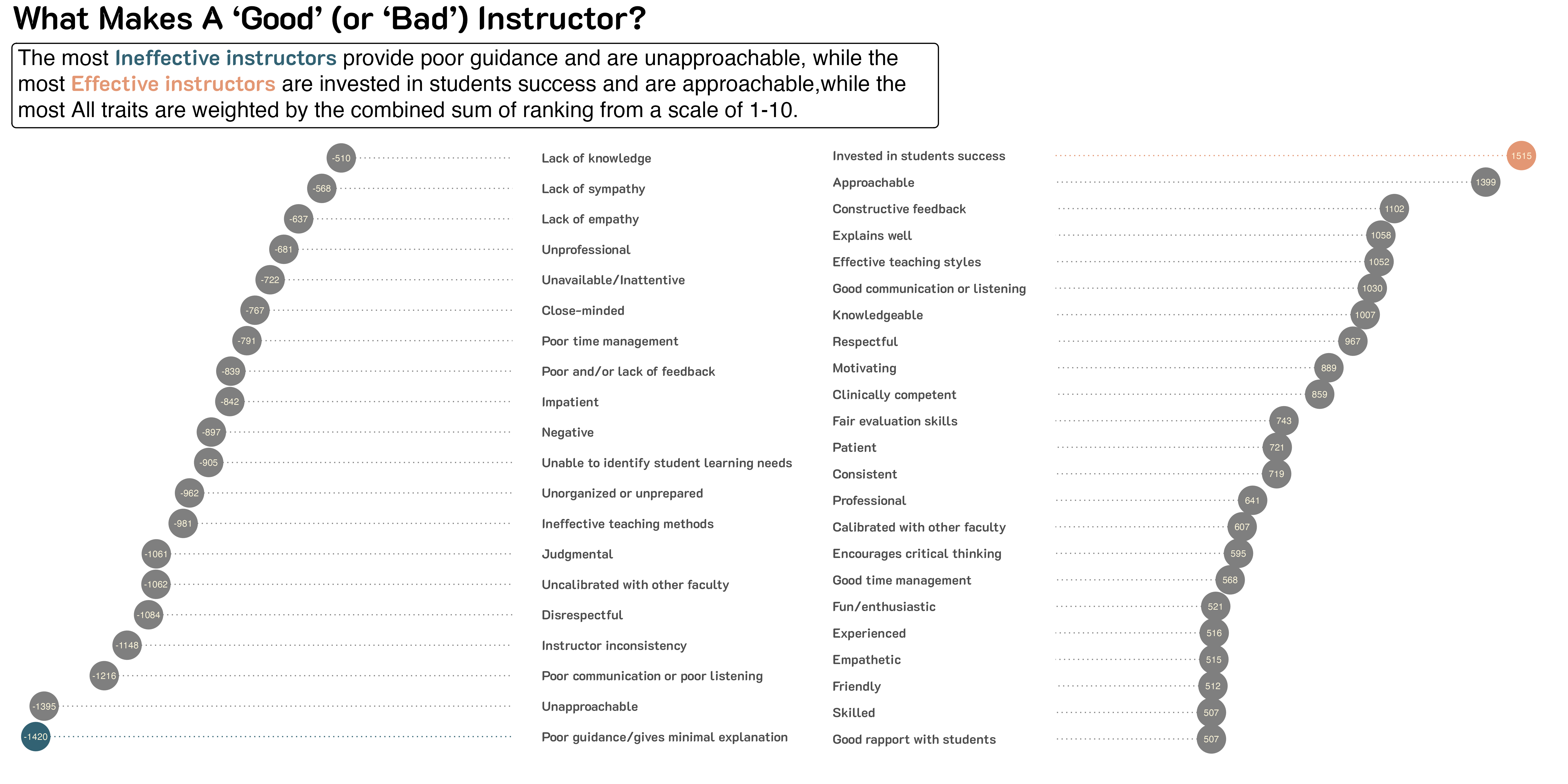
Next, all data was arranged so that a total weighting score could be applied to each trait. For example, if a trait was endorsed as being number 1 in terms of priority, it would be weighted as a 10.
For example: A set of 5 scores where Trait X is rated to be {1, 1, 1, 3, 5} would be converted to {10, 10, 10, 7, 5}. This would give Trait X a weighted ranking of 42. To delineate between effective and ineffective traits, all frequency counts in the ineffective traits were negated.
The traits for both effective and ineffective traits are compared by their respective weights and visualized only with traits over 500 weight.
Code
# Plot: Effectiveap1 <- at_cln_ttl |>filter(type =="Effective") |>filter(total >500) |>ggplot(aes(fct_reorder(traits,total),total)) +geom_segment(aes(x = traits, xend = traits,y = total, yend =0,color =ifelse(total ==max(total), "#E39774","grey50")),lty =3) +geom_point(size =12,aes(color =ifelse(total ==max(total),"#E39774","grey5 0"))) +theme_minimal() +coord_flip() +geom_text(aes(label = total),size =3,color ="cornsilk") +labs(x ="",y ="",color ="", ) +theme(plot.title.position ="plot",plot.title =element_markdown(size =15,face ="bold"),plot.subtitle =element_markdown(),panel.grid =element_blank(),axis.text.x =element_blank(),axis.text.y =element_text(hjust =0,face ="bold", size =12),legend.position ="none" ) +scale_color_identity() +ylim(0,1550)# Plot: Ineffectiveap2 <- at_cln_ttl |>filter(type =="Ineffective") |>filter(total <-500) |>ggplot(aes(fct_reorder(traits,total),total)) +geom_segment(aes(x = traits, xend = traits,y = total, yend =0,color =ifelse(total ==min(total), "#326273","grey50")),lty =3) +geom_point(size =12,aes(color =ifelse(total ==min(total),"#326273","grey5 0"))) +theme_minimal() +coord_flip() +geom_text(aes(label = total),size =3,color ="cornsilk") +labs(x ="",y ="",color ="", ) +theme(plot.title.position ="plot",plot.title =element_markdown(size =15,face ="bold"),plot.subtitle =element_markdown(),panel.grid =element_blank(),axis.text.x =element_blank(),axis.text.y =element_text(hjust =0,face ="bold",size =12),legend.position ="none" ) +scale_color_identity() +scale_x_discrete(position ="top")pl <- ap2 / ap1title_label <-"What Makes A 'Good' (or 'Bad') Instructor?"subtitle_label <-"The most <span style = 'color: #326273'>**Ineffective instructors**</span> provide poor guidance and are unapproachable, while the most <span style = 'color: #E39774'>**Effective instructors**</span> are invested in students success and are approachable,while the most All traits are weighted by the combined sum of ranking from a scale of 1-10."pl +plot_layout(ncol =2, nrow =1) +plot_annotation(title = title_label,subtitle = subtitle_label,theme =theme(plot.subtitle =element_textbox_simple(size =20,padding =margin(5.5, 0, 5.5, 5.5),margin =margin(1, 0, 5.5, 0),r = grid::unit(4,"pt"),width =unit(.6,"npc"),hjust =0,linewidth = .5,linetype =1, ),plot.title =element_markdown(face ="bold",size =30) ))
Sub-Themes
Sub-themes were classified based on previous work by Pizanis (2023). Traits were overall categorized into either Pedagogy, Affective, or Experience. The Table below shows the array of subthemes with a mix of ineffective and effective trait types. Effective traits are italicized and Ineffective traits have no text-face.
Code
subs <- at_cln_ttl |>mutate(subtheme =case_when( traits %in%c("Invested in students success","Approachable","Respectful","Motivating","Patient","Friendly","Empathetic","Fun/enthusiastic","Good rapport with students","Engaging","Sympathetic","Attentive","Unapproachable","Disrespectful","Judgmental","Lack of empathy","Lack of sympathy","Not engaging","Negative") ~"Affective", traits %in%c("Knowledgeable","Clinically competent","Professional","Experienced","Skilled","Self-awareness of strengths and weaknesses","Patient oriented", "Integrity","Unprofessional","Lack of knowledge","Lack of skill", "Poor patient interaction", "Low confidence", "Lack of experience", "Lack of integrity") ~"Expertise", traits %in%c("Constructive feedback", "Effective teaching styles", "Explains well", "Good communication or listening", "Fair evaluation skills", "Consistent", "Calibrated with other faculty", "Encourages critical thinking", "Good time management", "Available", "Inclusive", "Poor guidance/ gives minimal explanation", "Poor communication or poor listening", "Insturctor inconsistency", "Uncalibrated with other faculty", "Ineffective teaching methods", "Unorganized or unprepared", "Ineffective", "Impatient", "Poor and/or lack of feedback","Poor time management","Close-minded", "Unavailable/Inattentive", "Instructor inconsistency","Poor guidance/gives minimal explanation") ~"Pedagogical" ) )# Group by Subtheme and Splitall_st <- subs |>select(subtheme,traits,type) |>arrange(type) |>group_by(subtheme) |>group_split()# Pedagogyst1 <- all_st[[3]] |>select(traits) |>hux() |>map_italic(by_function(function(x) x %in% all_st[[3]][[2]][1:11]) )# Affectivest2 <- all_st[[1]] |>select(traits) |>hux() |>map_italic(by_function(function(x) x %in% all_st[[1]][[2]][1:12]) )# Expertisest3 <- all_st[[2]] |>select(traits) |>hux() |>map_italic(by_function(function(x) x %in% all_st[[2]][[2]][1:7]))# Combinestall <- st1 |>add_columns(c(st2$traits,rep("",3))) |>add_columns(c(st3$traits,rep("",8))) |>theme_article()# Renamestall[1,1:3] <-c("Pedagogy","Affective","Expertise")stall
Pedagogy
Affective
Expertise
Available
Approachable
Clinically competent
Calibrated with other faculty
Attentive
Experienced
Consistent
Empathetic
Integrity
Constructive feedback
Engaging
Knowledgeable
Effective teaching styles
Friendly
Professional
Encourages critical thinking
Fun/enthusiastic
Self-awareness of strengths and weaknesses
Explains well
Good rapport with students
Skilled
Fair evaluation skills
Invested in students success
Lack of experience
Good communication or listening
Motivating
Lack of integrity
Good time management
Patient
Lack of knowledge
Inclusive
Respectful
Lack of skill
Close-minded
Sympathetic
Low confidence
Impatient
Disrespectful
Poor patient interaction
Ineffective teaching methods
Judgmental
Unprofessional
Instructor inconsistency
Lack of empathy
Poor and/or lack of feedback
Lack of sympathy
Poor communication or poor listening
Negative
Poor guidance/gives minimal explanation
Not engaging
Poor time management
Unapproachable
Unavailable/Inattentive
Uncalibrated with other faculty
Unorganized or unprepared
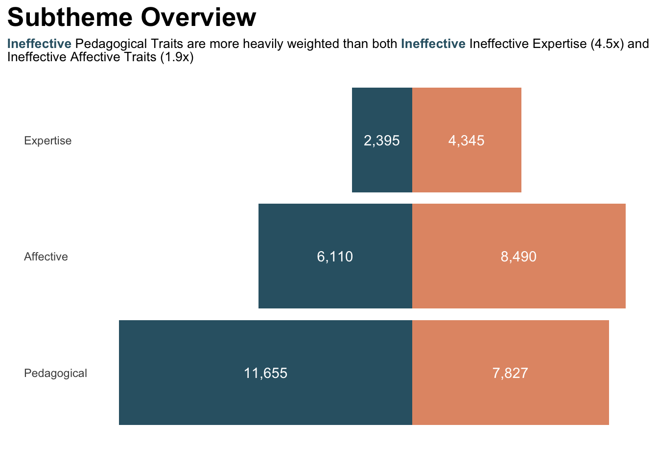
Sub-Theme Distribution
Pedagogy is the sub-theme category with the most number of items and the one category that weighted the heaviest in comparison to Expertise and Affectiveness.
Code
trait_master <- all_traits |>mutate(# Get Labels of Demographic variablesGender = sjlabelled::get_labels(all_traits$gender)[all_traits$gender],Year = sjlabelled::get_labels(all_traits$year)[all_traits$year],School = sjlabelled::get_labels(all_traits$school)[all_traits$school],Region = sjlabelled::get_labels(all_traits$geographical_region)[all_traits$geographical_region],Region =str_remove_all(Region, "\\(.*\\)"),Region =trimws(Region),Age = sjlabelled::get_labels(all_traits$age)[all_traits$age]) |> labelled::remove_labels() |>pivot_longer(cols = Approachable:`Not engaging`,names_to ="traits",values_to ="rating") |>mutate(subtheme =case_when( traits %in%c("Invested in students success","Approachable","Respectful","Motivating","Patient","Friendly","Empathetic","Fun/enthusiastic","Good rapport with students","Engaging","Sympathetic","Attentive","Unapproachable","Disrespectful","Judgmental","Lack of empathy","Lack of sympathy","Not engaging","Negative") ~"Affective", traits %in%c("Knowledgeable","Clinically competent","Professional","Experienced","Skilled","Self-awareness of strengths and weaknesses","Patient-oriented", "Integrity","Unprofessional","Lack of knowledge","Lack of skill", "Poor patient interaction", "Low confidence", "Lack of experience", "Lack of integrity") ~"Expertise", traits %in%c("Constructive feedback", "Effective teaching styles", "Explains well", "Good communication or listening", "Fair evaluation skills", "Consistent", "Calibrated with other faculty", "Encourages critical thinking", "Good time management", "Available", "Inclusive", "Poor guidance/gives minimal explanation", "Poor communication or poor listening", "Instructor inconsistency", "Uncalibrated with other faculty", "Ineffective teaching methods", "Unorganized or unprepared", "Ineffective", "Impatient", "Poor and/or lack of feedback","Poor time management","Close-minded", "Unavailable/Inattentive","Unable to identify student learning needs") ~"Pedagogical" ),w_rating =case_when( rating ==1~10, rating ==2~9, rating ==3~8, rating ==4~7, rating ==5~6, rating ==6~5, rating ==7~4, rating ==8~3, rating ==9~2, rating ==10~1 ) )p5 <- trait_master |>inner_join(trait_names, by =join_by(traits)) |>mutate(old =ifelse(str_detect(old, "^ef"), "Effective", "Ineffective")) |>rename(type = old) |>group_by(type, subtheme) |>summarize(total =sum(w_rating, na.rm =TRUE), .groups ="drop") |>mutate(total =ifelse(type =="Effective", total, -total)) |>ggplot(aes( subtheme, total,fill = type,label = scales::comma(abs(total)) )) +geom_bar(stat ="identity") +geom_text(aes(y = total /2), color ="white") +coord_flip() +theme_minimal() +scale_fill_manual(values =c("#E39774", "#326273")) +labs(x ="",y ="",fill ="Trait Type",title ="Subtheme Overview",subtitle ="<span style = 'color: #326273'>**Ineffective**</span> Pedagogical Traits are more heavily weighted than both <span style = 'color: #326273'>**Ineffective**</span> Ineffective Expertise (4.5x) and Ineffective Affective Traits (1.9x)" ) +theme(plot.subtitle =element_textbox_simple(size =10,lineheight =1,padding =margin(0, 0, 5, 0) ),plot.title.position ="plot",plot.title =element_text(size =20, face ="bold"),legend.position ="none",panel.grid =element_blank(),axis.text.y =element_text(hjust =0),axis.text.x =element_blank() )# Sort by Low to Highp5 +aes(x =fct_reorder(subtheme,total, .fun = min)) +labs(x ="")
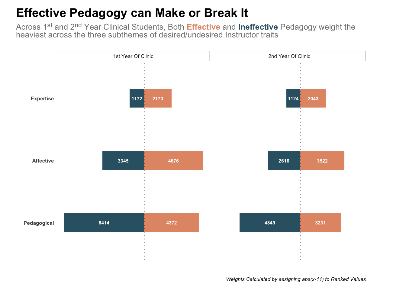
Sub-theme by Clinical Placement Year
Demographic data was collected including what year in clinical practice participants were currently in. Years included 1st and 2nd.
Code
trait_master |>inner_join(trait_names, by =join_by(traits)) |>mutate(old =ifelse(str_detect(old,"^ef"),"Effective","Ineffective")) |>rename(type = old) |>group_by(Year,type,subtheme) |>summarize(total =sum(w_rating, na.rm =TRUE),.groups ="drop") |>mutate(shift =ifelse(type =="Effective",total,-total),middle = shift/2,Year =str_to_title(Year)) |>filter(Year !="Other") |>ggplot(aes(fct_reorder(subtheme,shift),shift, fill = type)) +geom_bar(stat="identity",width = .3 ) +theme_minimal(base_size =8 ) +coord_flip() +scale_fill_manual(values =c("#E39774","#326273") ) +geom_hline(yintercept =0,alpha = .5,lty =3 ) +facet_grid(cols =vars(Year),switch ="y" ) +labs(y ="",x ="",fill ="Trait Type",title ="Effective Pedagogy can Make or Break It",subtitle ="Across 1<sup>st</sup> and 2<sup>nd</sup> Year Clinical Students, Both <span style = 'color: #E39774'>**Effective**</span> and <span style = 'color: #326273'>**Ineffective**</span> Pedagogy weight the heaviest across the three subthemes of desired/undesired Instructor traits<br>",caption ="<br>*Weights Calculated by assigning abs(x-11) to Ranked Values*" ) +theme(legend.position ="none",axis.text.x =element_blank(),plot.margin =margin(t =10, r =50, b =10, l =20, unit ="pt"),panel.grid =element_blank(),plot.title.position ="plot",plot.title =element_text(size =15,face ="bold"),plot.subtitle =element_textbox_simple(size =10, lineheight =1, padding =margin(0,0,5,0),color ="grey50" ),plot.caption =element_markdown(),axis.text.y =element_text(face ="bold"),strip.background =element_rect(fill ="white", color ="black", linewidth = .2) ) +geom_text(aes(label =abs(shift), y = middle),color ="white",fontface ="bold",size =2.1 )
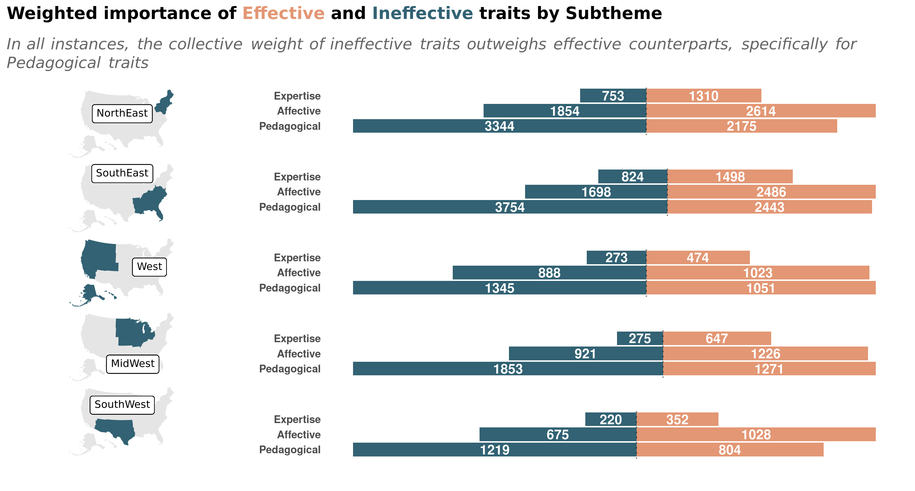
Subthemes by Demographic Region
Demographic data was collected including what region of the United States participants came from. Regions included the MidWest, NorthEast, SouthEast, SouthWest, and West. Grand weighted scores for each sub-theme is illustrated below.
Demographics
The table below shows the demographic make-up of the participants. Regional data has been modified to only show the region name and not the states that compose it.
Code
demo <- all_traits |>select(gender,year,age,school,geographical_region) |>mutate(# Get Labels of Demographic variablesGender = sjlabelled::get_labels(all_traits$gender)[all_traits$gender],Year = sjlabelled::get_labels(all_traits$year)[all_traits$year],School = sjlabelled::get_labels(all_traits$school)[all_traits$school],Region = sjlabelled::get_labels(all_traits$geographical_region)[all_traits$geographical_region],Region =str_remove_all(Region, "\\(.*\\)"),Region =trimws(Region),Age = sjlabelled::get_labels(all_traits$age)[all_traits$age],Year =ifelse(str_detect(Year,"1st"),"First Year of Clinic","Second Year of Clinic"),School =ifelse(str_detect(School,"2"),"Community College or Two Year College","University or Four Year College"))# Apply Custom Functiongen <-discrete_tab(demo,"Gender")year <-discrete_tab(demo,"Year")school <-discrete_tab(demo,"School")geo <-discrete_tab(demo,"Region")age <-discrete_tab(demo,"Age")demo_hux <- gen |>add_rows(year) |>add_rows(school) |>add_rows(geo) |>add_rows(age) demo_hux |>set_align(col =1, value ="left") |>set_align(col =2:4, value ="center") |>set_number_format(2) |>set_col_width(c(.5,.5,.5,.5))