12  Two Factor Between Subject ANOVA

Recall the way that the ANOVA is formatted:

onefact <- 
  data.frame(groups = rep(c("Control","Treatment 1", "Treatment 2"), each = 20),
             score = c(rnorm(20,10),rnorm(20,15),rnorm(20,22)))

head(onefact)
   groups     score
1 Control 10.996546
2 Control  9.753324
3 Control 10.896292
4 Control 10.103684
5 Control  9.839047
6 Control 10.289613

We have three independent variables, or conditions, control, treatment 1 and treatment 2. We have one dependent variable, some idea of “score” or our dependent variabe.

The ANOVA is analyzed through the use of the aov function. Remember to save the analysis as a model so you can use it later if you need to do any post-hoc tests/unplanned comparisons.

onefact.mod <- aov(score~groups, data=onefact)

summary(onefact.mod)
            Df Sum Sq Mean Sq F value Pr(>F)    
groups       2 1518.4   759.2    1132 <2e-16 ***
Residuals   57   38.2     0.7                   
---
Signif. codes:  0 '***' 0.001 '**' 0.01 '*' 0.05 '.' 0.1 ' ' 1

This produces a sum of squares and mean squares for the between subjects factor, groups. It also produces a sum of squares and mean squares for the within subjects factor, also called the residuals, or the error.

From this we get one F-value.

The current design will not help us too much so we need to move on to another design, the two factor between subjects ANOVA.

The set-up is mostly the same:

twofact.df <- 
   data.frame(Gender=c(rep("Male", 30), rep("Female",30)),
              Diet= c(rep(c("Diet 1", "Diet 2"), 30)),
              Count=c(rnorm(30,28,2),rnorm(30,35,2)))
 twofact.df
   Gender   Diet    Count
1    Male Diet 1 26.48755
2    Male Diet 2 31.47564
3    Male Diet 1 28.13363
4    Male Diet 2 25.52771
5    Male Diet 1 24.35407
6    Male Diet 2 27.30847
7    Male Diet 1 26.00746
8    Male Diet 2 27.23500
9    Male Diet 1 28.00621
10   Male Diet 2 30.59714
11   Male Diet 1 28.84651
12   Male Diet 2 26.09762
13   Male Diet 1 21.83050
14   Male Diet 2 28.54673
15   Male Diet 1 27.43047
16   Male Diet 2 28.28352
17   Male Diet 1 27.36914
18   Male Diet 2 27.61665
19   Male Diet 1 25.72843
20   Male Diet 2 27.47735
21   Male Diet 1 28.34706
22   Male Diet 2 31.35059
23   Male Diet 1 29.50067
24   Male Diet 2 30.68563
25   Male Diet 1 24.61919
26   Male Diet 2 30.43092
27   Male Diet 1 26.79289
28   Male Diet 2 28.97912
29   Male Diet 1 30.27497
30   Male Diet 2 32.21793
31 Female Diet 1 34.84730
32 Female Diet 2 37.88996
33 Female Diet 1 31.06975
34 Female Diet 2 37.13204
35 Female Diet 1 37.94516
36 Female Diet 2 36.45220
37 Female Diet 1 31.66604
38 Female Diet 2 32.81201
39 Female Diet 1 32.45473
40 Female Diet 2 34.68988
41 Female Diet 1 33.72885
42 Female Diet 2 36.71112
43 Female Diet 1 37.14371
44 Female Diet 2 34.77879
45 Female Diet 1 40.20775
46 Female Diet 2 35.38483
47 Female Diet 1 33.96295
48 Female Diet 2 34.31245
49 Female Diet 1 33.92102
50 Female Diet 2 34.10081
51 Female Diet 1 36.67242
52 Female Diet 2 34.16263
53 Female Diet 1 30.79080
54 Female Diet 2 35.64382
55 Female Diet 1 37.68124
56 Female Diet 2 35.86778
57 Female Diet 1 32.47617
58 Female Diet 2 38.06221
59 Female Diet 1 32.60325
60 Female Diet 2 39.29878

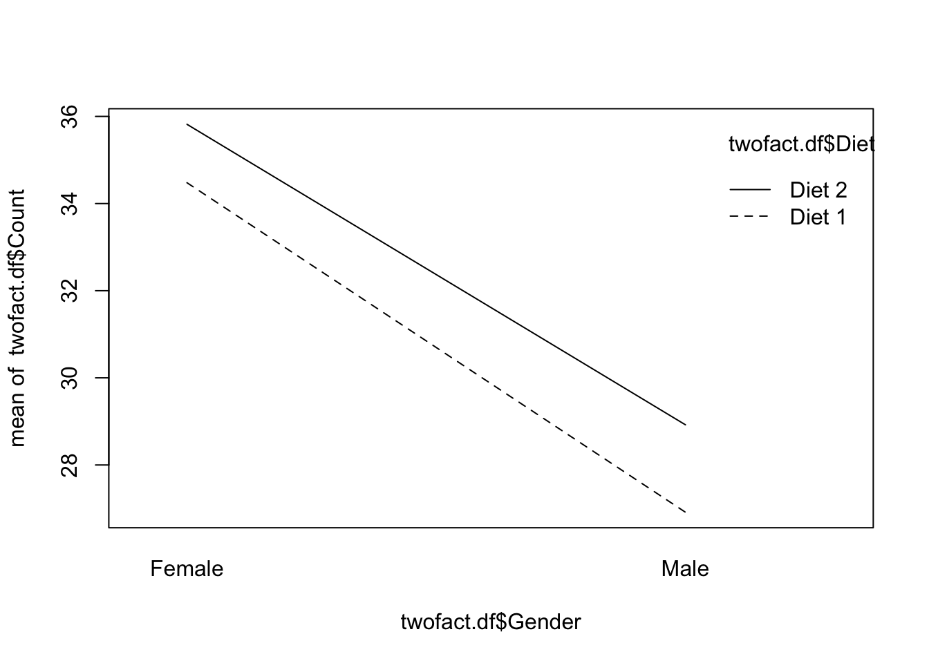
We can see that there are two levels of the independent variable (gender) and two levels of the independent variable (Diet) and one dependent variable, count.

From this we will generate four sums of squares and four mean squares. - Sum of Squares for Factor A - Sum of Squares for Factor B - - Sum of Squares for the interaction between A and B - Sum of Squares within, or Error, or residual.

Analyzing the data just uses one more term:

twofact.mod<-aov(Count~Gender*Diet,data = twofact.df)
summary(twofact.mod)
            Df Sum Sq Mean Sq F value  Pr(>F)    
Gender       1  784.2   784.2 154.215 < 2e-16 ***
Diet         1   42.1    42.1   8.269 0.00569 ** 
Gender:Diet  1    1.7     1.7   0.326 0.57031    
Residuals   56  284.8     5.1                    
---
Signif. codes:  0 '***' 0.001 '**' 0.01 '*' 0.05 '.' 0.1 ' ' 1

What do these results look like?

In order to plot these relationships we can use interaction.plot.

interaction.plot(twofact.df$Gender,twofact.df$Diet, twofact.df$Count)

df <- 
  data.frame(iv1 = rep(c("Level 1","Level 2"),each=2,20),
             iv2 = rep(c("Level 1","Level 2"),each=1,40),
             scored = rnorm(80,c(15,20,30,40)))


length(df$iv1)
[1] 80
length(df$iv2)
[1] 80
length(df$scored)
[1] 80
summary(aov(scored~iv1*iv2,data = df))
            Df Sum Sq Mean Sq F value Pr(>F)    
iv1          1   6175    6175  8327.3 <2e-16 ***
iv2          1   1129    1129  1522.0 <2e-16 ***
iv1:iv2      1    139     139   187.2 <2e-16 ***
Residuals   76     56       1                   
---
Signif. codes:  0 '***' 0.001 '**' 0.01 '*' 0.05 '.' 0.1 ' ' 1
interaction.plot(df$iv1,df$iv2,df$scored)

12.1 Two Factor Within Subjects ANOVA

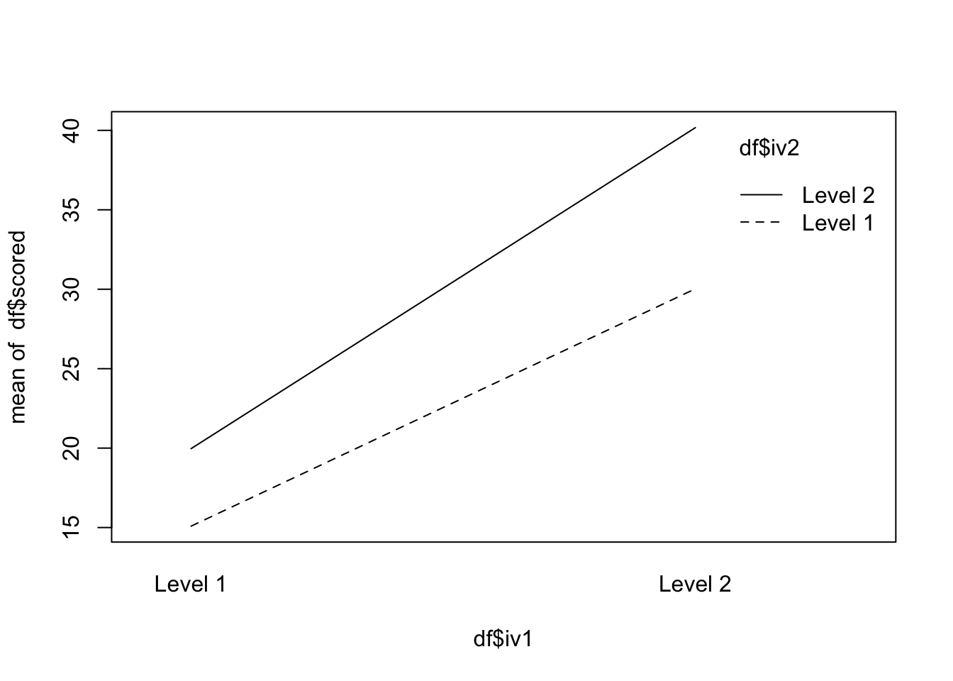
In a Two Factor Between Subjects ANOVA, a particular participant is only ever in one condition or group or treatment level.

In a Two Factor Within Subjects ANOVA, a particular participant is in each condition or group or treatment level.

Setting this data up uses the same principles as we have learned before.

The one major difference in the set-up of the data is that there is now a variable of the subject itself.

When we had a between subjects design, each participant was unique, with a within deisgn, each participant experiences every aspect of the experiment so it is reasonable that they may have an effect on the experiment itself.

Here is a sample dataset:

set.seed(1234)

within_anova <- 
  data.frame(subject=rep(1:10,4),
             groups=rep(c("pre","post","post 1", "post 2"),each = 10),
             score=rnorm(40,c(20,30,40,70)))

head(within_anova)
  subject groups    score
1       1    pre 18.79293
2       2    pre 30.27743
3       3    pre 41.08444
4       4    pre 67.65430
5       5    pre 20.42912
6       6    pre 30.50606

It would be helpful if we could see the means of each group, and plot those means.

For this, we will use a new function called tapply. This applies a specified function to whatever variables you provide in the arguments.

To get the means:

within_means <- 
  tapply(within_anova$score,within_anova$groups,mean)

within_means
    post   post 1   post 2      pre 
42.88183 36.61205 42.23381 36.61684 

To get the standard deviations:

within_sd <- 
  tapply(within_anova$score,within_anova$groups,sd)

within_sd
    post   post 1   post 2      pre 
20.47817 18.96593 20.24584 18.49391 

For now, we will only use tapply in order to get the means.

Here is how we will plot the means:

plot(within_means, pch=19,
      xlab = "Treatments",
      ylab = "Survey Score",
      main = "Means of Survey Score by Treatment")

Performing the ANOVA requires two new terms: Error and the Subject factor.

The model that the ANOVA should resemble looks like this:

aov(DV~IV+Error(Subjects))

From here it is important to note that your IV *must* be a factor.

With this in mind, you should run the function levels(Grouping Variable) or factor(Grouping Variable.)

If the first function returns NULL, use the second function.

Putting all of this together gives us the following:

within_anova.mod <- aov(score~groups+Error(subject),data = within_anova)
summary(within_anova.mod)

Error: subject
          Df Sum Sq Mean Sq F value Pr(>F)
Residuals  1  113.9   113.9               

Error: Within
          Df Sum Sq Mean Sq F value Pr(>F)
groups     3    355   118.4   0.303  0.823
Residuals 35  13665   390.4               

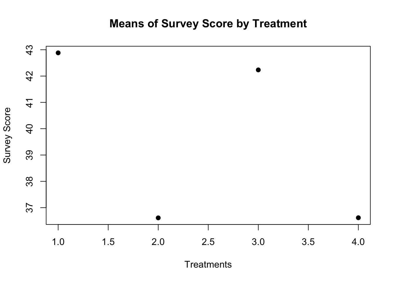
When reporting these findings, you will ignore the subject variable and report the F-value for the grouping variable.

This particular finding should be reported as follows:

\(F(3,35) = .303, p >.05\)

The results of a one-factor within subjects ANOVA revealed that there does not appear to be any effect of treatment on survey score.

12.2 Effect Sizes

Most times you will want to report effect sizes for your experiment. Effect sizes help to tell you how much of your effect is due to your manipulation.

In this example, there does not appear to be an effect at all, but we will compute an effect size anyways.

We will be using the \(\omega^2\) effect size estimate.

The formula is as follows:

\[\omega^2 = \frac{SS_B-(k-1)(MS_W)}{SS_T-MS_W}\]

or

\[\omega^2 = \frac{SS_{Effect}-(k-1)(MS_{Within})}{SS_{Total}-MS_{Within}}\]

There is no R function that reports \(\omega^2\), so we will do this by hand.

\(\omega^2 = \frac{355-(4-1)(390.4)}{14020-390.4}\)

\(\omega^2 = -.059\)

This effect size is negative because our effect was not significant, but it is still important for you to see how to get these numbers!