One-Sample T-Test

PSY 348: Lecture 9

Dave Brocker

Farmingdale State College

Recap

How did we get here?

straighten

Measurement

Measuring abstract concepts

Variables

Types and scales

show_chart

The Normal Curve

Probability from z-scores

groups

Sampling Theory

Distribution of sample means

If we can estimate the probability that a sample mean came from a particular distribution, can we also estimate whether it came from the null or the alternative hypothesis?

From Probability to Decision-Making

Once we know how likely a sample mean is to occur, we can begin to make decisions about what that likelihood means.
We introduced two competing ideas:

Null hypothesis \(H_0\)

No real difference or effect.

Alternative hypothesis \(H_1/H_A\)

A true difference or effect exists.

Because samples vary, we can never be 100% certain, only confident to a degree.

Errors in Estimation

Type I and II Error

That degree of confidence is defined by \(\alpha\) (alpha), our threshold for error when rejecting \(H_0\).
\(\beta\) (beta) is the probability of missing a real effect (failing to reject \(H_0\) when \(H_1\) is true).

Type I Error (\(\alpha\)): Finding a difference that isn’t really there. (False Positive)

Type II Error (\(\beta\)): Missing a difference that actually exists. (False Negative)

The Truth Table

	\[H_0\text{ True}\]	\[H_0\text{ False}\]
Decision Outcomes in Hypothesis Testing
\[\text{Reject }H_0\]	\[\text{Type I Error }(\alpha)\]	\[\text{Correct Decision}\\1-\beta\]
\[\text{Fail to Reject } H_0\]	\[\text{Correct Decision}\\1-\alpha\]	\[\text{Type II Error } (\beta)\]

Alpha and Beta

Seeing the two errors

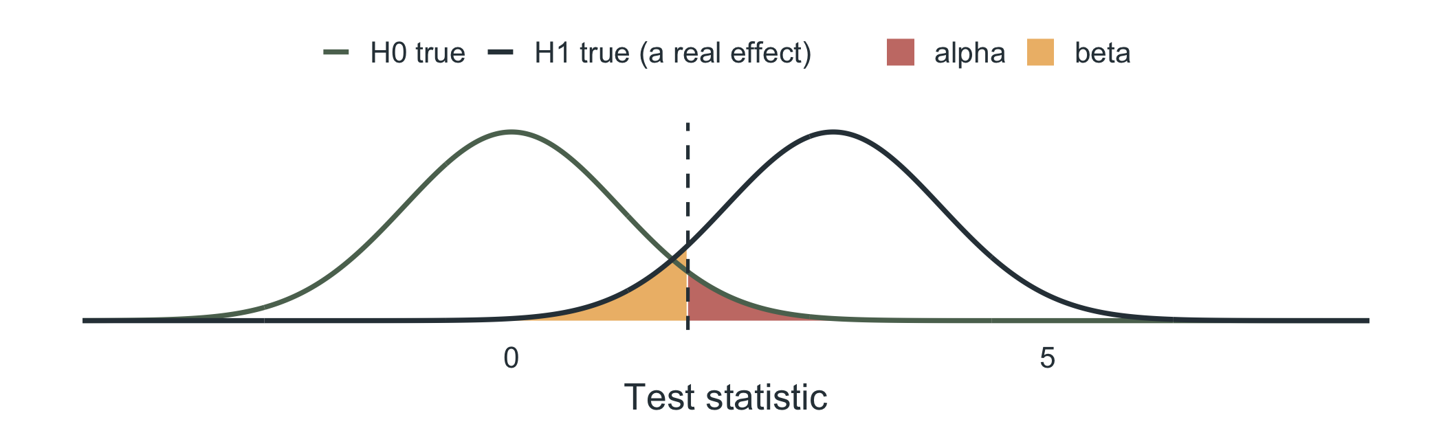
The dashed line is the critical value: beyond it we reject \(H_0\).
\(\alpha\) (red): a true null gets rejected (Type I error). \(\beta\) (orange): a real effect is missed (Type II error).
Power is \(1 - \beta\): the chance of detecting a real effect.

Why Compare Means?

We often want to test whether a sample mean differs from a known population mean.
The one-sample t-test helps determine if the sample mean is significantly different from the hypothesized population mean.

school

Exam scores

Class average vs. a national average of 75

timer

Reaction times

Average vs. a published 250 ms standard

linear_scale

Scale midpoints

Ratings vs. the scale midpoint

Why Not z?

From z to t

In lecture 8 we computed \(z = \dfrac{\bar{x} - \mu}{\sigma / \sqrt{n}}\), which needs the population standard deviation \(\sigma\).
In practice we almost never know \(\sigma\), so we substitute the sample’s \(s\).
But \(s\) changes from sample to sample, especially when \(n\) is small. That is extra uncertainty the normal curve does not account for.
So the sampling distribution has heavier tails than the normal curve: the t-distribution. A result must be more extreme to count as unusual.

Why Not z?

Same \(\alpha = .05\), bigger cutoff for small samples

Two-tailed critical values:

1.96

z (\(\sigma\) known)

2.09

t, \(df = 19\) (\(n = 20\))

2.78

t, \(df = 4\) (\(n = 5\))

The smaller the sample, the more the t cutoff moves away from the z cutoff. With large \(n\), they are nearly identical.

The t-test

Three types, three cases

One-Sample

\(t=\dfrac{\bar{x}-\mu}{s/\sqrt{n}}\)

Paired-Samples

\(t=\dfrac{\bar{D}}{s_D/\sqrt{n}}\)

Independent-Samples

\(t = \dfrac{\bar{x}_1 - \bar{x}_2}{\sqrt{s_p^2\left(\frac{1}{n_1} + \frac{1}{n_2}\right)}}\)

\(s_p^2 = \dfrac{(n_1 - 1)s_1^2 + (n_2 - 1)s_2^2}{n_1 + n_2 - 2}\)

We use the sample SD (\(s\)) to estimate the standard error (\(s/\sqrt{n}\)), since \(\sigma\) is usually unknown. \(s_D\) is the SD of the difference scores and \(s_p^2\) is the pooled variance.
The critical value depends on the degrees of freedom: \(df = n - 1\) (one-sample, paired) or \(n_1 + n_2 - 2\) (independent).

The Sample SD, \(s\)

\[s = \sqrt{\dfrac{\sum (x_i - \bar{x})^2}{n-1}}\]

Numerator: each score’s squared distance from the mean, added up
Denominator: \(n-1\), then take the square root
For \(s_D\), use each person’s difference score \(D\) in place of \(x\)
We use \(s\) because \(\sigma\) is usually unknown (if \(\sigma\) were known, we would use \(\sigma/\sqrt{n}\) and a z-test instead)

The t-distribution

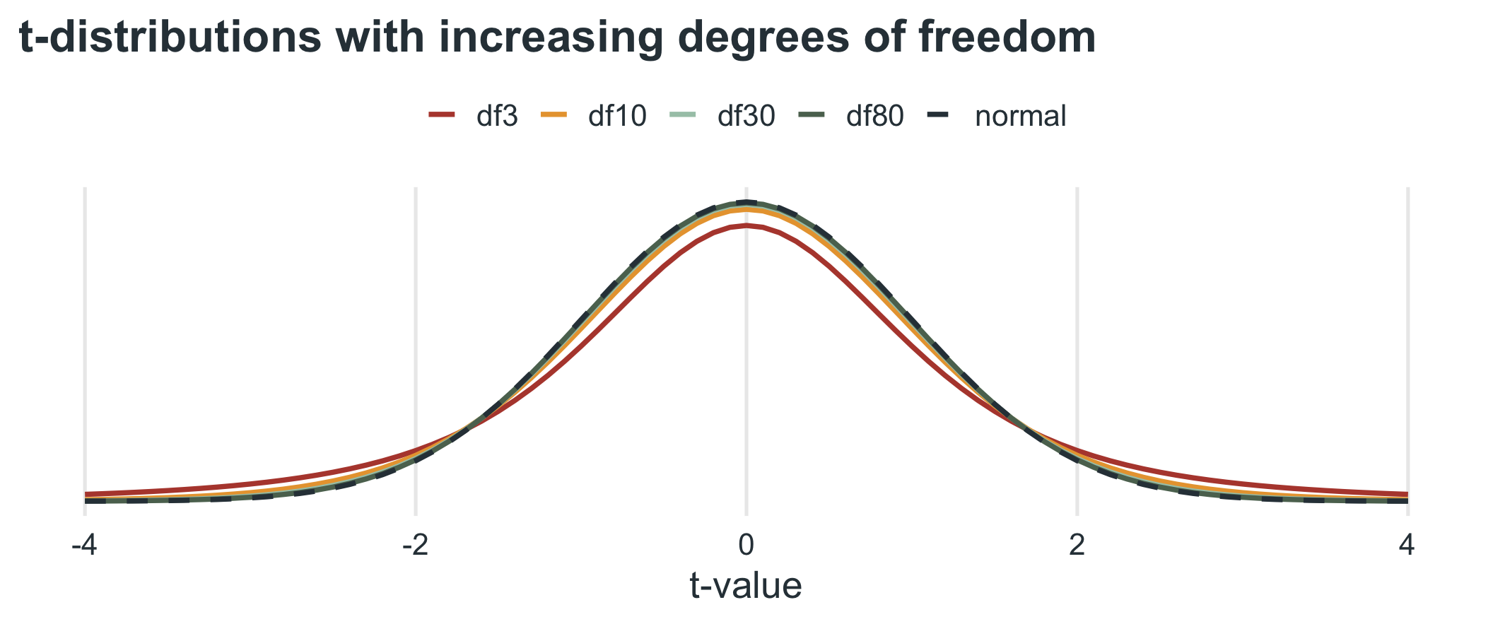
The t-distribution has heavier tails than the normal curve when df is small, because \(s\) is only an estimate of \(\sigma\).
As df grows, the t-distribution approaches the normal curve.

Assumptions of the One-Sample t-Test

Assumptions

The data are continuous (interval or ratio scale).
The sample is randomly selected.
The data are normally distributed (or the sample size is large enough for the Central Limit Theorem to apply).

The One-Sample t-Test Formula

One-Sample t-Test

\(\large{t = \dfrac{\color{blue}{\bar{x}} - \mu}{\color{orange}{s}/\sqrt{n}}}\)

\(\color{blue}{\bar{x}}\) = sample mean
\(\mu\) = population mean (null hypothesis value)
\(\color{orange}{s}/\sqrt{n}\) = the standard error (SE), estimated from the sample: \(s\) is the sample SD and \(n\) the sample size
\(s = \sqrt{\dfrac{\sum (x_i - \bar{x})^2}{n-1}}\) = sum of squared deviations from the mean, divided by \(n-1\), then square-rooted

Hypothesis Testing Steps

Four steps

Set hypotheses: define both the null and alternative.
Collect sample data: use the appropriate sampling method and collect the needed data.
Compute the t-statistic: conduct the correct t-test.
Compare to the critical value: use the t-statistic, sample size (df), and alpha level to determine statistical significance. Equivalently, compare the p-value to \(\alpha\).

Reading the t-Table

Critical values by degrees of freedom

Excerpt of the t-table (critical values)
df	One-tailed .05 (two-tailed .10)	One-tailed .025 (two-tailed .05)	One-tailed .005 (two-tailed .01)
15	1.753	2.131	2.947
19	1.729	2.093	2.861
24	1.711	2.064	2.797
29	1.699	2.045	2.756
∞ (z)	1.645	1.960	2.576

Find your df (\(n - 1\) for a one-sample test), then the column for your \(\alpha\) and tails. If \(|t|\) is beyond the critical value, reject \(H_0\) (here \(2.68 > 2.093\)).
In R: qt(.975, df = 19) returns 2.093 (the upper 2.5% cutoff).

Hypothesis Testing Steps

Manual: hypotheses and data

20 students have a mean exam score of 78 (SD = 5). Does the class differ from the national average of 75?

1. Set hypotheses

\(H_0\): The average exam score is 75 (\(\mu = 75\)).
\(H_A\): The average exam score is not 75 (\(\mu \neq 75\)).

2. Collect sample data

\(n = 20\), \(\color{blue}{\bar{x}} = 78\), \(\color{orange}{s} = 5\)

Hypothesis Testing Steps

Manual: test and decide

3. Compute the t-statistic

\(t = \dfrac{78 - 75}{\frac{5}{\sqrt{20}}} = \dfrac{3}{1.118} = 2.68\)

4. Compare to the critical value

At \(\alpha = .05\) (two-tailed) and \(df = 19\): \(t_{critical} = \pm 2.093\).
Since \(2.68 > 2.093\), we reject \(H_0\).

Hypothesis Testing Steps

Programmatic

one_sample.R

# For Reproducibility
set.seed(20)

n = 20   # sample size
m = 78   # sample mean
mu = 75  # population mean (H0)
s = 5    # sample SD

# Simulate data, then rescale so the sample has exactly mean 78 and SD 5
dat <- rnorm(n)
dat <- m + s * (dat - mean(dat)) / sd(dat)

t.test(dat, mu = mu)


    One Sample t-test

data:  dat
t = 2.6833, df = 19, p-value = 0.01471
alternative hypothesis: true mean is not equal to 75
95 percent confidence interval:
 75.65993 80.34007
sample estimates:
mean of x 
       78

Hypothesis Testing Steps

Programmatic: by hand and the critical value

check.R

# By hand
(m - mu) / (s / sqrt(n))

[1] 2.683282

# Critical value (two-tailed, alpha = .05)
qt(.975, df = n - 1)

[1] 2.093024

Reporting Results

APA-style

A one-sample t-test was conducted to compare exam scores to the national average of 75. Results showed a significant difference, t(19) = 2.68, p = .015, indicating that students scored significantly higher than the national average (M = 78, SD = 5).

What kind of test?
What is being compared?
Is it significant?
What are the test results?

Reporting Results

APA-style

A one-sample t-test was conducted to compare exam scores to the national average of 75. Results showed a significant difference, t(19) = 2.68, p = .015, indicating that students scored significantly higher than the national average (M = 78, SD = 5).

What kind of test? one-sample t-test
What is being compared? exam scores to the national average
Is it significant? significant difference
What are the test results? t(19) = 2.68, p = .015

Interpreting Results

Sample summary table

A significant result (\(p < .05\)) suggests that the sample mean is different from the population mean.
A non-significant result (\(p > .05\)) means we fail to reject \(H_0\) (insufficient evidence of a difference).

	M	t	p	df	conf.low	conf.high	alternative
One Sample t-test	78	2.683	0.015	19	75.66	80.34	two.sided

Visualizing Data

Scores against the national average

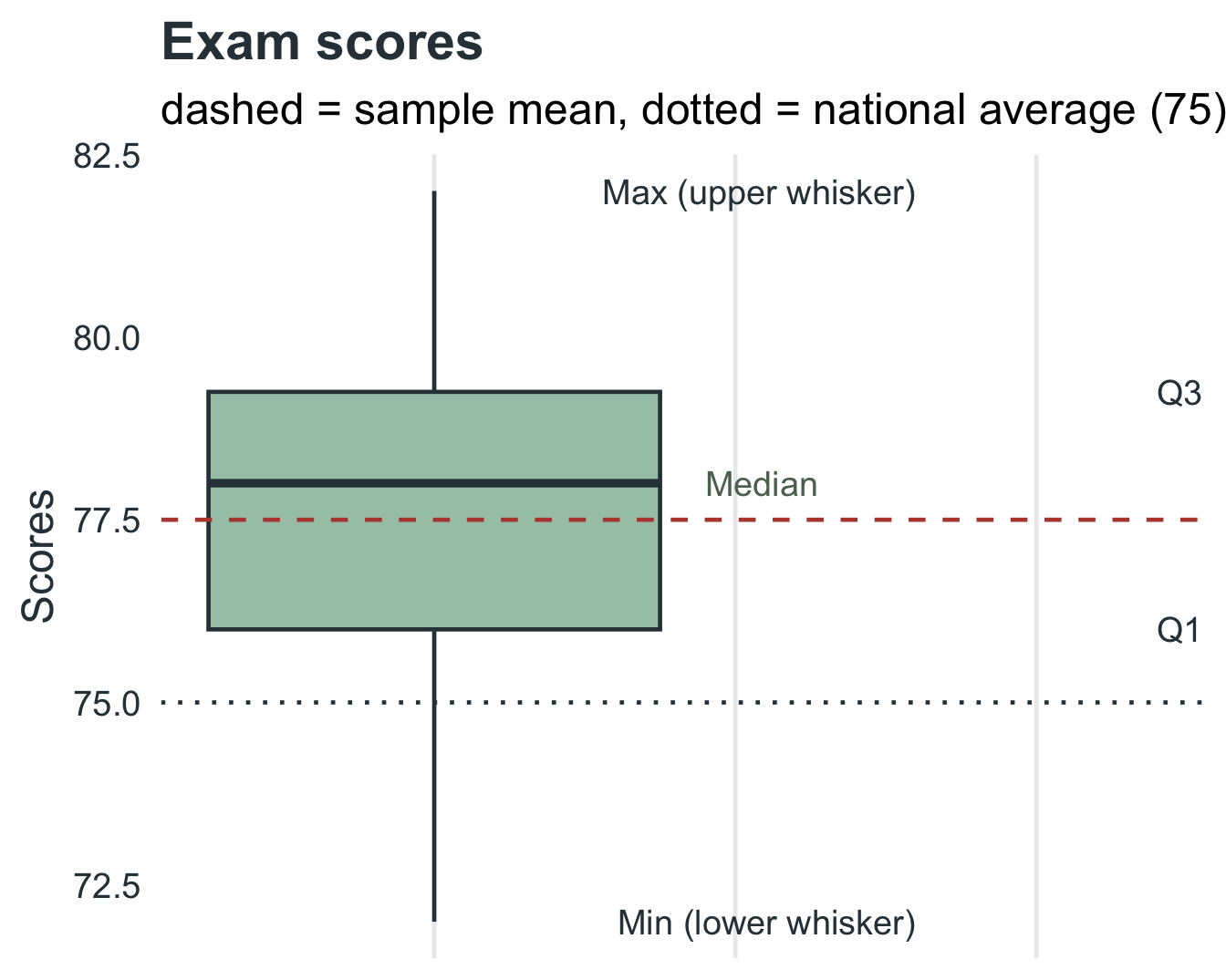
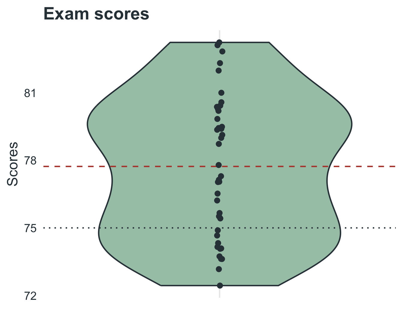
Exam Scores vs. National Average

Hypotheses

A professor wants to test if students in their class scored differently from the national average of 75 on an exam. A sample of 25 students has a mean score of 78 with a standard deviation of 10.

Null Hypothesis (\(H_0\)): \(\mu = 75\) (no difference)
Alternative Hypothesis (\(H_A\)): \(\mu \neq 75\) (scores differ)

Exam Scores vs. National Average

Manual

Compute t

\(t = \dfrac{\color{blue}{\bar{x}} - \mu}{\frac{\color{orange}{s}}{\sqrt{n}}} = \dfrac{78 - 75}{\frac{10}{\sqrt{25}}} = \dfrac{3}{2} = 1.5\)

Decide

For \(df = 24\) (\(25 - 1\)), the critical value at \(\alpha = .05\) (two-tailed) is \(\pm 2.064\). Since \(|t| = 1.5 < 2.064\), we fail to reject \(H_0\).

Exam Scores vs. National Average

Programmatic

exam_scores.R

# For Reproducibility
set.seed(131)

# Simulate data, then rescale so the sample has exactly mean 78 and SD 10
x <- rnorm(25)
x <- 78 + 10 * (x - mean(x)) / sd(x)

t.test(
  x,
  # The population mean to test against
  mu = 75
  )


    One Sample t-test

data:  x
t = 1.5, df = 24, p-value = 0.1467
alternative hypothesis: true mean is not equal to 75
95 percent confidence interval:
 73.8722 82.1278
sample estimates:
mean of x 
       78

APA Reporting

A one-sample t-test was conducted to determine whether students’ exam scores differed from the national average (\(\mu\) = 75). Results were not statistically significant, t(24) = 1.50, p = .147, indicating that students performed similarly to the national average (M = 78, SD = 10).

Daily Coffee Consumption

Hypotheses

A coffee company claims that people drink an average of 3 cups of coffee per day. A researcher samples 16 individuals, finding a mean of 2.5 cups and a standard deviation of 1 cup.

Null Hypothesis (\(H_0\)): \(\mu = 3\)
Alternative Hypothesis (\(H_A\)): \(\mu < 3\) (people drink less)

Daily Coffee Consumption

Manual

Compute t

\(t = \dfrac{2.5 - 3}{1 / \sqrt{16}} = \dfrac{-0.5}{0.25} = -2.0\)

Decide

For \(df = 15\) (\(16 - 1\)), the critical t-value for a one-tailed test at \(\alpha = .05\) is \(-1.753\). Since \(-2.0 < -1.753\), we reject \(H_0\).

Daily Coffee Consumption

Programmatic

coffee.R

# For Reproducibility
set.seed(131)

# Simulate data, then rescale so the sample has exactly mean 2.5 and SD 1
x <- rnorm(16)
x <- 2.5 + 1 * (x - mean(x)) / sd(x)

t.test(
  x,
  # The value claimed by the company
  mu = 3,
  # Our alternative is directional: fewer than 3 cups
  alternative = "less"
  )


    One Sample t-test

data:  x
t = -2, df = 15, p-value = 0.03197
alternative hypothesis: true mean is less than 3
95 percent confidence interval:
     -Inf 2.938263
sample estimates:
mean of x 
      2.5

APA Reporting

A one-sample t-test was conducted to test whether daily coffee consumption was lower than the reported average of 3 cups. Results showed a significant difference, t(15) = -2.00, p = .032 (one-tailed), suggesting that people consume significantly fewer cups of coffee per day than reported (M = 2.5, SD = 1).

Sleep Duration Among College Students

Hypotheses

A health researcher believes college students sleep less than 7 hours per night. A sample of 30 students reports a mean of 6.5 hours with a standard deviation of 1.2 hours.

Null Hypothesis (\(H_0\)): \(\mu = 7\)
Alternative Hypothesis (\(H_A\)): \(\mu < 7\)

Sleep Duration Among College Students

Manual

Compute t

\(t = \dfrac{6.5 - 7}{1.2 / \sqrt{30}} = \dfrac{-0.5}{0.219} = -2.28\)

Decide

For \(df = 29\), the critical t-value for a one-tailed test at \(\alpha = .05\) is \(-1.699\). Since \(-2.28 < -1.699\), we reject \(H_0\).

Sleep Duration Among College Students

Programmatic

sleep.R

# For Reproducibility
set.seed(728)

# Simulate data, then rescale so the sample has exactly mean 6.5 and SD 1.2
x <- rnorm(30)
x <- 6.5 + 1.2 * (x - mean(x)) / sd(x)

t.test(
  x,
  # The value we are testing against
  mu = 7,
  # Our alternative is directional: less than 7 hours
  alternative = "less"
  )


    One Sample t-test

data:  x
t = -2.2822, df = 29, p-value = 0.015
alternative hypothesis: true mean is less than 7
95 percent confidence interval:
    -Inf 6.87226
sample estimates:
mean of x 
      6.5

APA Reporting

A one-sample t-test was conducted to test whether college students sleep fewer than 7 hours per night. Results were statistically significant, t(29) = -2.28, p = .015 (one-tailed), indicating that students get significantly less sleep than the recommended amount (M = 6.5, SD = 1.2).