Hypothesis Testing, Pt 2
Lecture 10
Dave Brocker
Farmingdale State College
Review
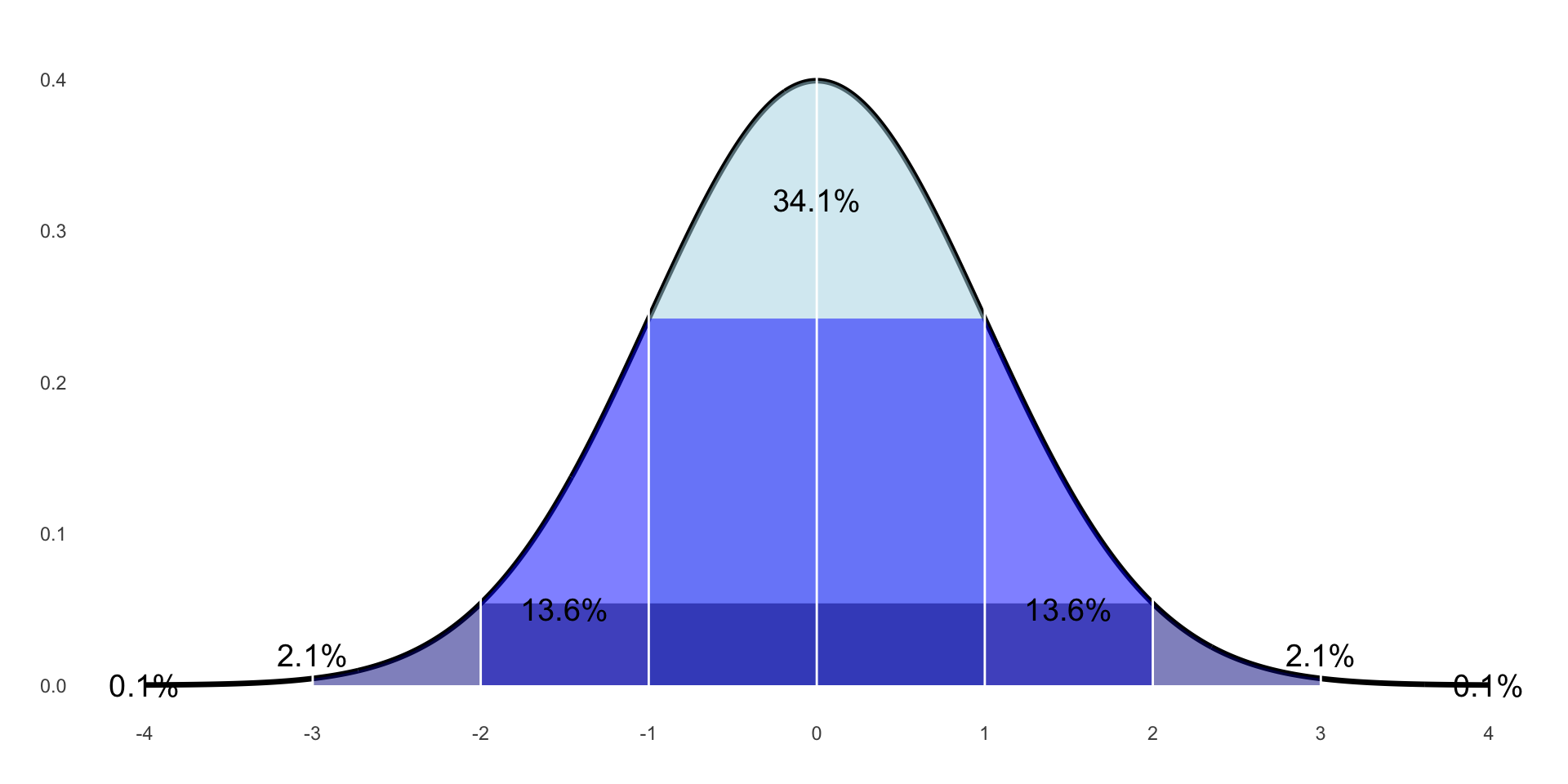
Sampling Theory
If we took infinite samples of a population, the mean of each sample taken would be a Sample Mean – like how each student collect 500 responses about TV show ratings and took the average of those 500 responses.
What we get if we put all the sample means together; we assume it’s a normal distribution.
Sampling theory
Each value in this distribution represents the average of 1 sample, a Sample Mean.
Sampling theory
There are about 10,000 students at Farmingdale State College.
Each of the 25 of us recruits a sample of 400 students.
We ask every single FSC student to rate their sense of belonging on FSC campus on a scale of 1 (I don’t belong at all) to 10 (I belong completely).
We each calculate the average response from our own sample of 400.
Sampling Theory
Just Making Sure…
P-Values
Yeah Can I Get Uhhhhh
Professor Brocker gives 100 students caffeinated coffee and another 100 students decaf. He then has them complete a stats exam.
P-Values
Yeah Can I Get Uhhhhh
Professor Brocker gives 100 students caffeinated coffee and another 100 students decaf. He then has them complete a stats exam.
P-Values
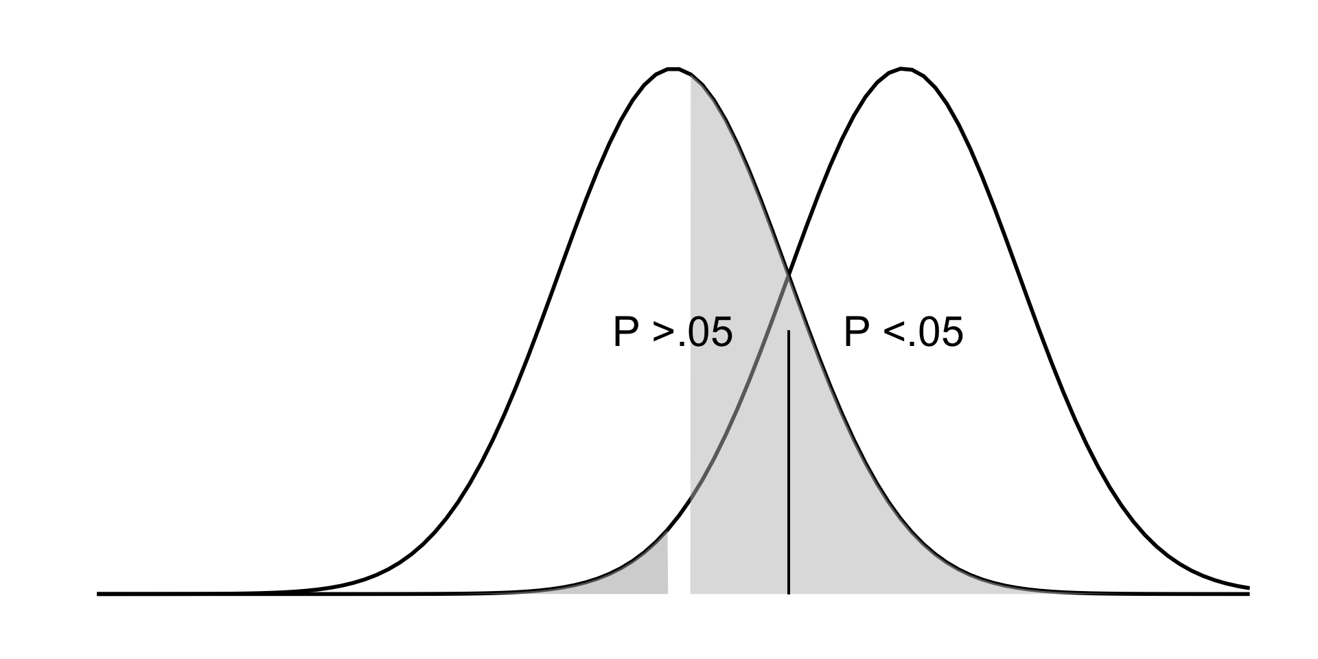
The p-value tells us if the mean of the experimental group is far enough away from the control group mean that we can be confidence it belongs to a theoretical non-null distribution.
P-values and confidence intervals
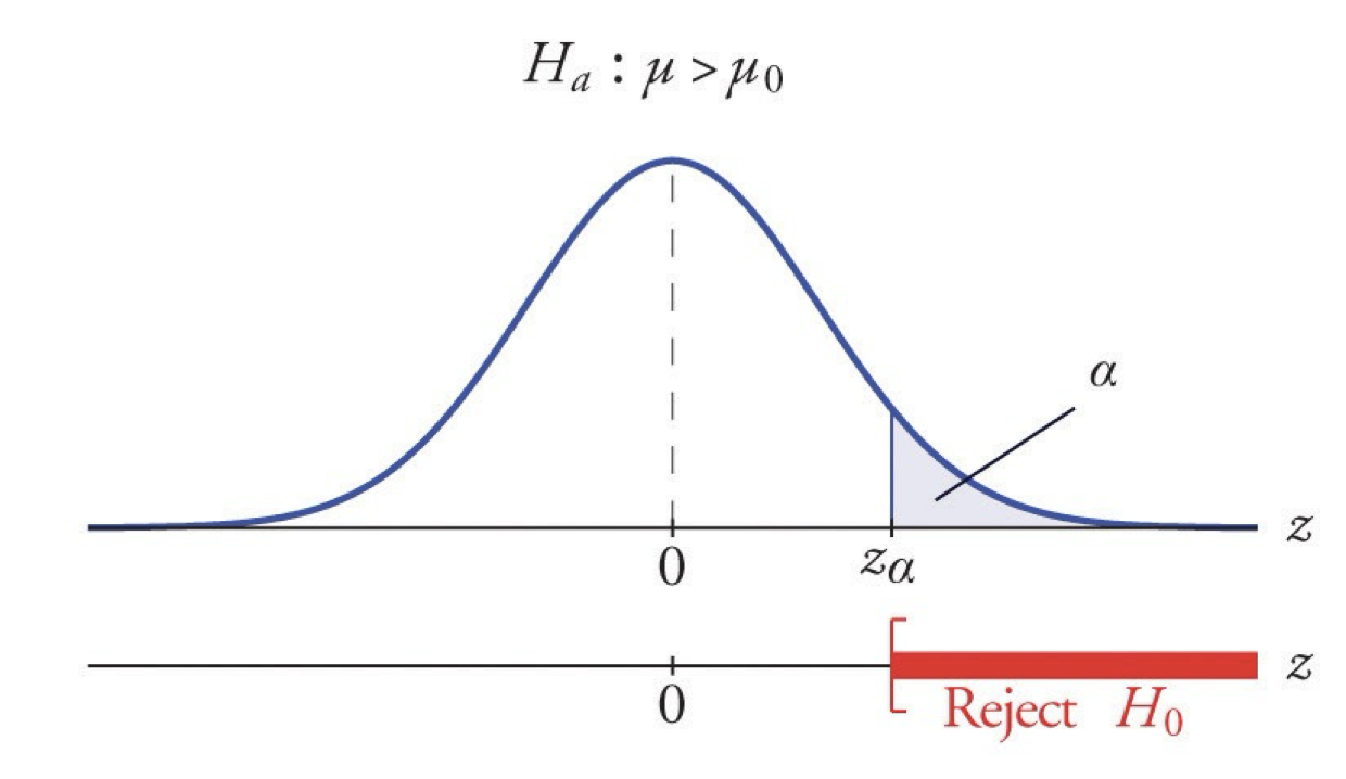
Finding in terms of the null hypothesis
If there is a significant difference between the groups, p will be smaller than 0.05.
If p < (less than) 0.05, the difference is significant, we Reject \(H_0\).
If p > (greater than) 0.05, the difference is NOT significant, we Fail to Reject \(H_0\).
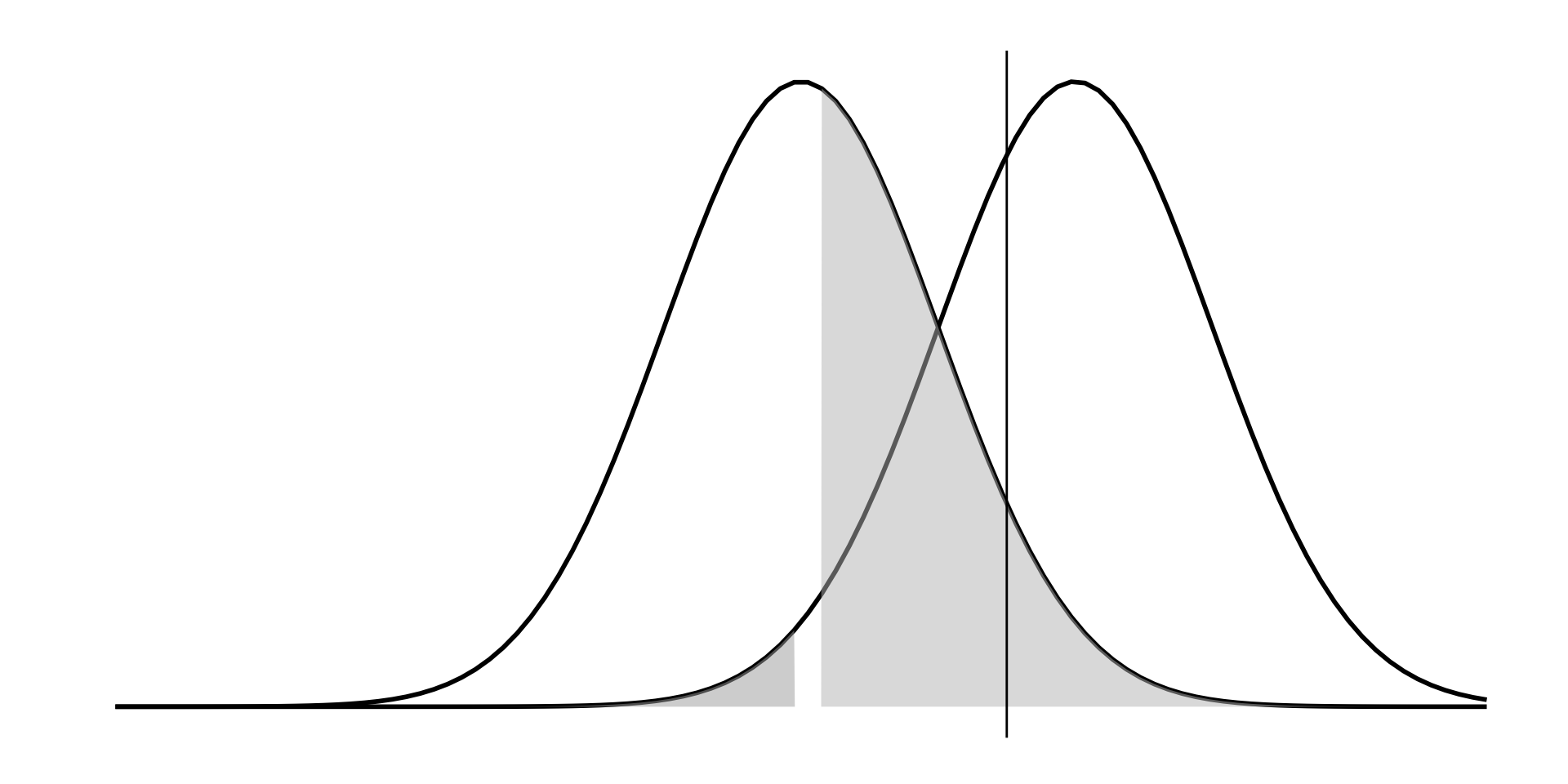
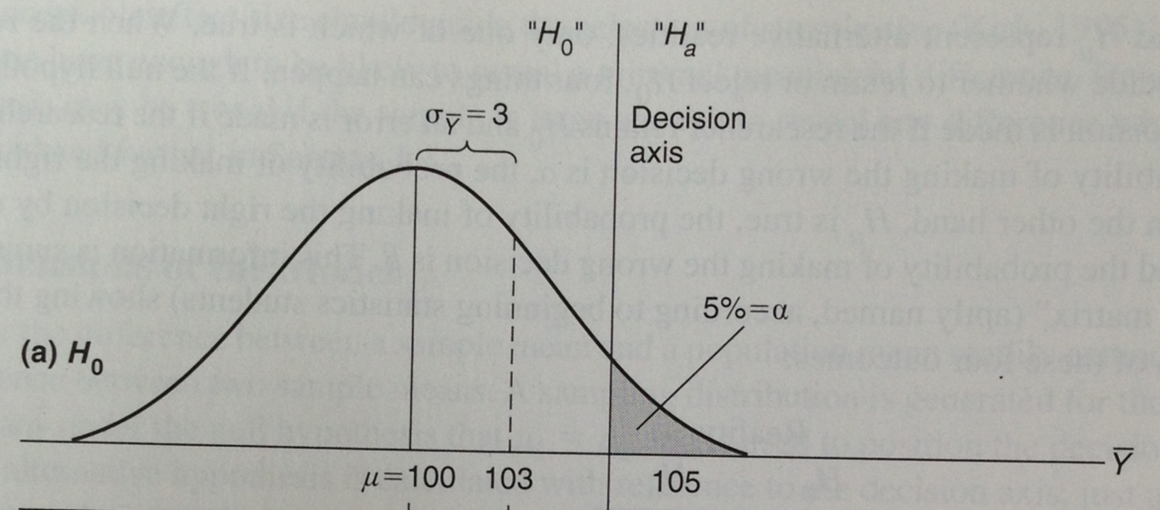
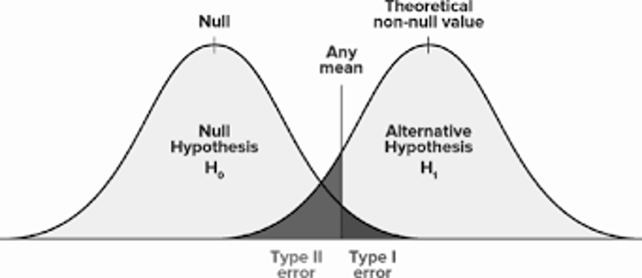
Error (\(\beta\))
How often are we okay with making a mistake?
Types of Errors
Visual Aid
Error
How often are we okay with making a mistake?
- It’s better to make a Type 2 Error than a Type 1.
- Type 1 kills people
- Type 2 kills careers
- We want to minimize the chance of committing a Type 1 Error.
Error & Alpha
We accept a 5% chance of committing a Type 1 Error.
- We set alpha (\(\alpha\)) to
5% or 0.05
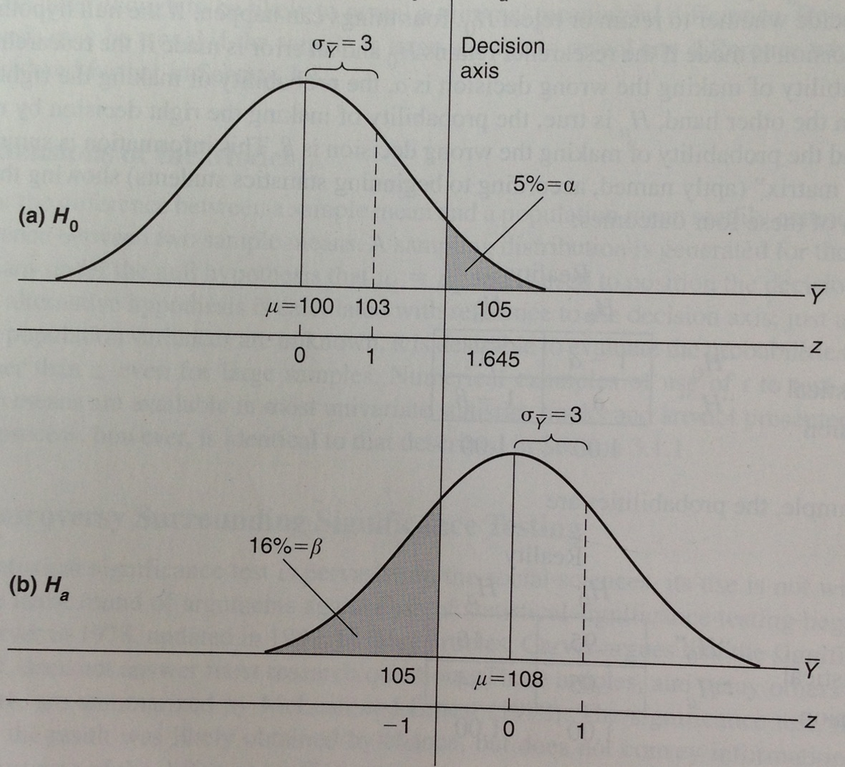
Beta
We set alpha at 5% (0.05), meaning we are okay with making a Type 1 Error (false positive) 5% of the time.
As a result, beta gets set at 16%, meaning we have a 16% chance of committing Type 2 Error (false negative).
Alpha and Beta
Example
![]()
Error and Alpha and Beta
| Fail to Reject \(H_0\) |
Correct Decision \(1-\alpha\) |
Incorrect Decision
Type II Error
\(\beta\) |
| Reject \(H_0\) |
Incorrect Decision
Type I Error
\(\alpha\) |
Correct Decision
\(1-\beta\) |
Null Hypothesis: \(H_0\)
States that nothing will happen while also naming of the variables (independent and dependent).
- The Null Hypothesis is written as \(H_0\)
Alternative hypothesis: \(H_1|H_A\)
A testable prediction of what will happen in our experiment that names of the variables (independent and dependent) and clearly contrasts the groups.
- The Alternative Hypothesis is written as \(H_1\)
Hypothesis testing
![]()
P-values and confidence intervals
If there is a significant difference between the groups, p will be smaller than 0.05.
If p = .032…
If p = .045…
If p = .050…
Findings in terms of the null hypothesis
If p < (less than) 0.05, the difference is significant, we Reject \(H_0\).
If p > (greater than) 0.05, the difference is NOT significant, we Fail to Reject \(H_0\).
Alpha & beta
![]()
Alpha & beta
\(\alpha\) and \(\beta\)
Alpha: The probability of committing a Type 1 Error.
- We set \(\alpha\) to
0.05
Beta: The probability of committing a Type 2 Error.
- When \(\alpha\) =
0.05, the resulting \(\beta\) = 0.16
Alpha & beta
![]()
Alpha and Beta and Power
![]()
Alpha & beta & power
![]()
Alpha & beta & power
![]()
Alpha & Beta & Power
![]()
Alpha & beta & Power
Alpha: The probability of committing a Type 1 Error.
- We set \(\alpha\) to
0.05
Beta: The probability of committing a Type 2 Error.
- When \(\alpha\) =
0.05, the resulting \(\beta\) = 0.16
Power: Ability of the researcher to accurately detect a difference between groups
- If \(\alpha\) =
0.05, \(\beta\) = 0.16, and the resulting power = 0.84
Alpha & Beta & Power
Power
Power refers to the ability of the researcher to accurately detect a difference between groups.
When we assume a normal distribution, we assume power will be about 0.84 or 84%.
Power is dependent on Effect Size.
Effect Size
Effect size in statistics refers to the strength of the relationship between two variables in a population.
- Cohen’s \(d\)
- Coefficient of Determination \(R2\)
- Omega Hat Squared | Eta Hat Squared
- \(\hat{\omega}^2\)
- \(\hat{\eta}\)
Effect Size Example
Does caffeine decrease the amount of time it takes to solve a puzzle?
Effect Size Example
Does caffeine decrease the amount of time it takes to solve a puzzle?
Caffeine versus no caffeine
Effect Size Example
Does caffeine decrease the amount of time it takes to solve a puzzle?
Strength of the relationships between caffeine and task speed
- How much does caffeine actually impact task speed?
Effect size Example
Does caffeine decrease the amount of time it takes to solve a puzzle?
Effect size
The strength of the relationship between two variables in a population.
Effect size tells us how much one variable actually impacts the other.
Effect size:
Cohen’s d
Effect size in statistics refers to the strength of the relationship between two variables in a population.
Cohen’s d gives us a standardized measure of effect size:
Cohen’s d
Cohen’s d is calculated by subtracting the mean of the experimental group from the mean of the control group and dividing it by the “pooled standard deviation.”
The pooled standard deviation refers to the average SD across the 2 groups.
\(d = \frac{M_2-M_1}{\sqrt{\frac{SD_1^2\ +\ SD_2^2}{2}}}\)
Cohen’s d
Understanding the Terms
\(d = \frac{M_2-M_1}{\sqrt{\frac{SD_1^2\ +\ SD_2^2}{2}}}\)
\(d = \frac{\text{Control Group Mean}-\text{Experimental Group Mean}}{\sqrt{\text{Pooled Variance}}}\)
Effect size
In psychology, we are often dealing with effect sizes that are small (d = 0.3).
- A smaller effect size is harder to detect.
Alpha & beta & power
When the effect size is small, the hypothetical alternative distribution is closer to the null distribution.
![]()
Effect size
What can we do to increase power when an effect size is small?