Sampling Theory

PSY 348: Lecture 8

Dave Brocker

Farmingdale State College

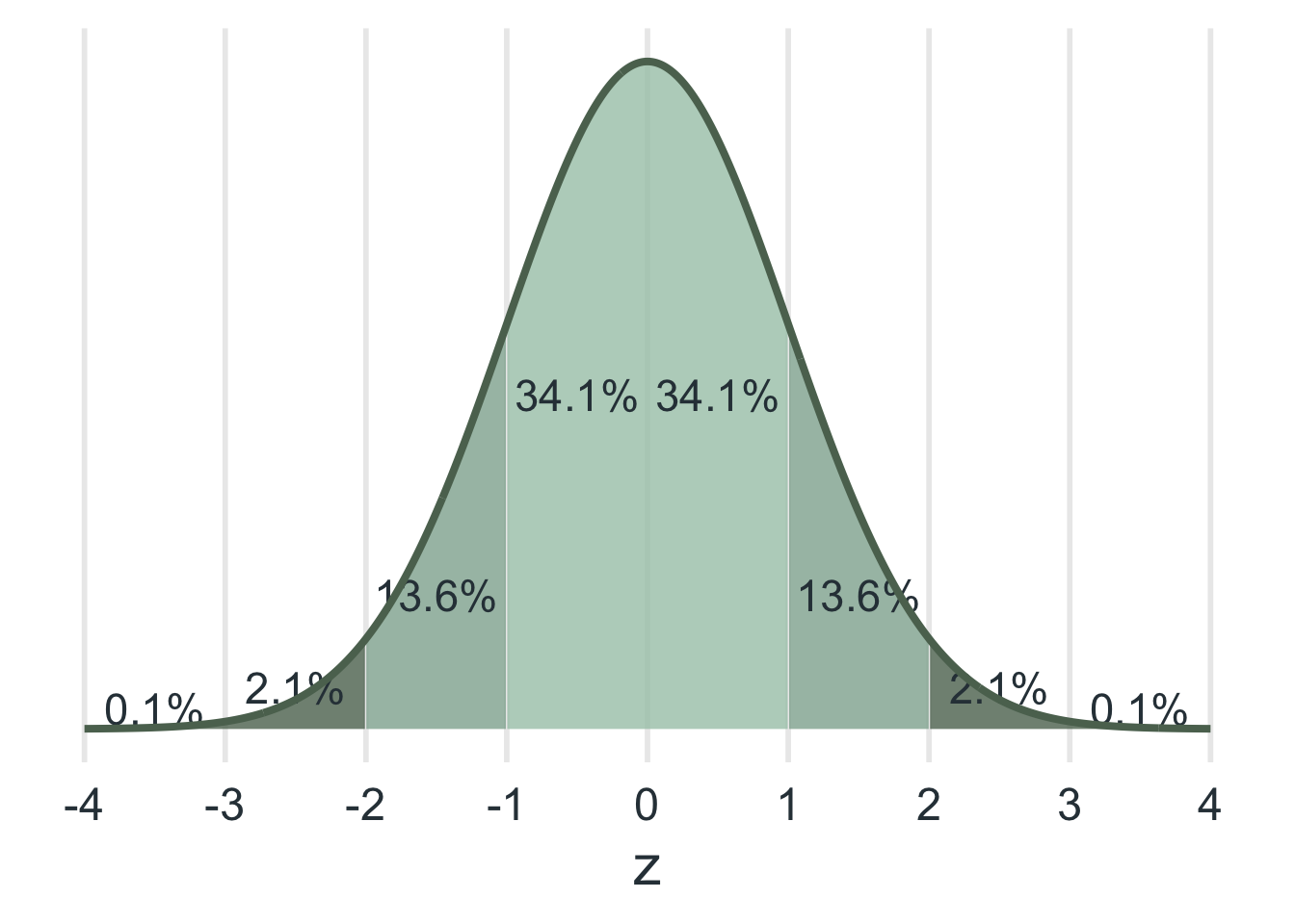
Normal Distribution

Four properties

• Shaped like a bell (“bell curve”).

• Symmetric.

• Unimodal.

• The mean = median = mode.

Statistics

Two goals

Descriptive Statistics

• Goal: describe the sample
• Examples: mean, standard deviation

Inferential Statistics

• Goal: use the sample to make inferences about the population
• Examples: t-test, ANOVA, regression

Sampling Theory

The Dark Study

Professor Brocker still wants to know how much adults in the US enjoy the Netflix Original, Dark. He has unlimited funds to study this very important research question. He hires 30 students to collect the data. Each student has to collect 500 responses to the following question:

Sampling Theory

The Question

On a scale of 1 (I hate it with my entire being) to 10 (I believe in my soul that Dark is the best show ever made), how much do you enjoy Dark?

Sampling Theory

Thirty Samples

• Each student asks 500 people how much they enjoy the Netflix Original Dark.

• How many people did the class ask in total?

  • \(30 \times 500 = 15{,}000\)

set.seed(348)

# 30 students each rate 500 people on the 1-10 scale
replicate(30, mean(pmin(pmax(round(rnorm(500, 6.6, 1.5)), 1), 10))) |>
  (\(m) tibble(Sample = paste0("S", 1:30), `Sample Mean` = m))() |>
  gt() |>
  fmt_number(columns = `Sample Mean`, decimals = 3) |>
  tab_options(table.width = pct(60), table.font.size = 22) |>
  opt_row_striping() |>
  opt_interactive(page_size_default = 8)

Sampling Theory

Sample Means

• Once each of you collects 500 responses, you calculate the average answer, the mean of your sample.

• \(\bar{x}_1 = \dfrac{x_1 + x_2 + x_3 + \cdots + x_{500}}{500}\)

• One mean per sample: \(\bar{x}_1, \bar{x}_2, \ldots, \bar{x}_{30}\).

Sampling Theory

Sample Mean

Sample Mean

The mean of one sample. A different sample of the same size gives a (slightly) different sample mean.

Sampling Theory

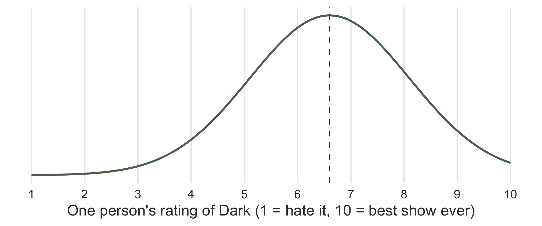
Here is our ratings data

Each point on this curve is one person’s rating.

Sampling Theory

What can we do with sample means?

• We could calculate the mean of the sample means.

• We could calculate the standard deviation of the sample means.

• With 30 samples we only get an approximation. To get the exact answer, we would need every possible sample of 500 people, and that is theoretical.

  • We imagine it for the sake of sampling theory.

Sampling Distribution

Definition

Sampling Distribution

The theoretical distribution of a statistic (here, the mean) across every possible sample of the same size \(n\) from the population.

Sampling Distribution

Same center, very different spread

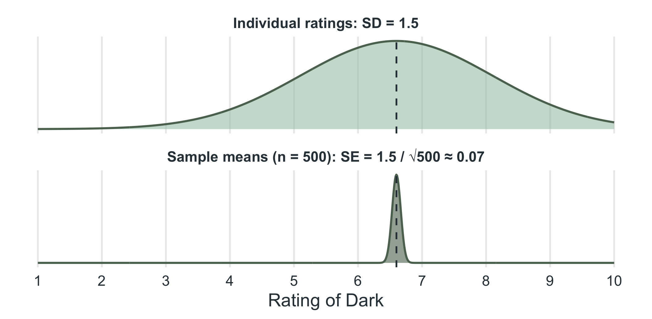
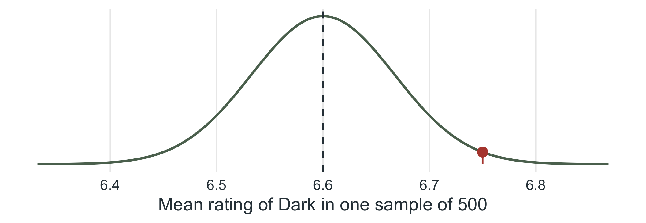
Both curves are centered on \(\mu = 6.6\). The top curve is a distribution of people. The bottom curve is a distribution of sample means, so it is much narrower.

Sampling Distribution

One value = one sample mean

• Each value in this distribution no longer represents one person.

• Each value represents the mean of one sample of 500 people.

Sampling Distribution

Standard error

Standard Error

The standard deviation of the sampling distribution of the mean: \(SE = \dfrac{\sigma}{\sqrt{n}}\), where \(\sigma\) is the population standard deviation and \(n\) is the sample size.

Standard Error

Bigger samples, narrower sampling distribution

\(\sigma = 1.5\) in every case; only \(n\) changes.

0.21

\(n = 50\)

0.07

\(n = 500\)

0.02

\(n = 5{,}000\)

• \(\sigma\) describes how spread out individual scores are.

• \(SE\) describes how spread out sample means are.

New Terminology

Sample and population symbols

• Sample mean \(\bar{x}\) (written \(M\) in APA-style papers) and sample SD \(s\) describe a sample.

• \(\mu\) (pronounced “mew”) is the population mean.

• \(\sigma\) is the population standard deviation.

• \(SE\) is the standard deviation of the sample means.

Term	Symbol	Formula
Sample Mean	\[\bar{x}\] or \[M\]	\[\frac{\sum x_i}{n}\]
Sample SD	\[s\]	\[\sqrt{\frac{\sum (x_i - \bar{x})^2}{n-1}}\]
Population Mean	\[\mu\]	\[\frac{\sum X_i}{N}\]
Population SD	\[\sigma\]	\[\sqrt{\frac{\sum (X_i - \mu)^2}{N}}\]
Standard Error	\[SE\]	\[\frac{\sigma}{\sqrt{n}}\]

Reading the Symbols

• \(\sum\) means “add up all the scores”
• \(n\) is the sample size and \(N\) is the population size
• We divide by \(n-1\) (not \(n\)) when computing \(s\) because the sample mean was estimated from the same data

Probability

Individuals first

• What percentage of participants rated Dark with a z-score of 2 or higher?

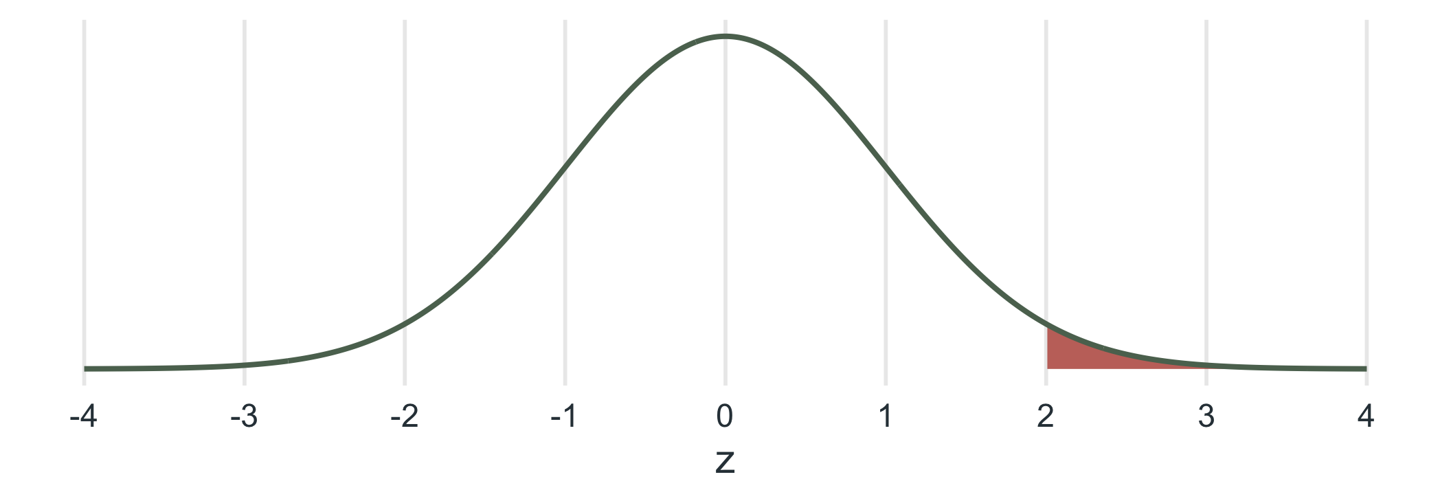
• About 2.3% of participants (\(1 - .9772 = .0228\)).

Probability

Now sample means

• This is the distribution of sample means from adults in the US. What is the probability that a sample has a mean with a z-score of 2 or higher?

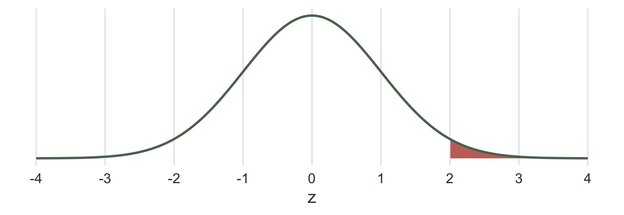
• Same curve, same area, new meaning: only about 2.3% of samples would produce a mean this high.

Central Limit Theorem

Why can we use the normal curve?

Central Limit Theorem

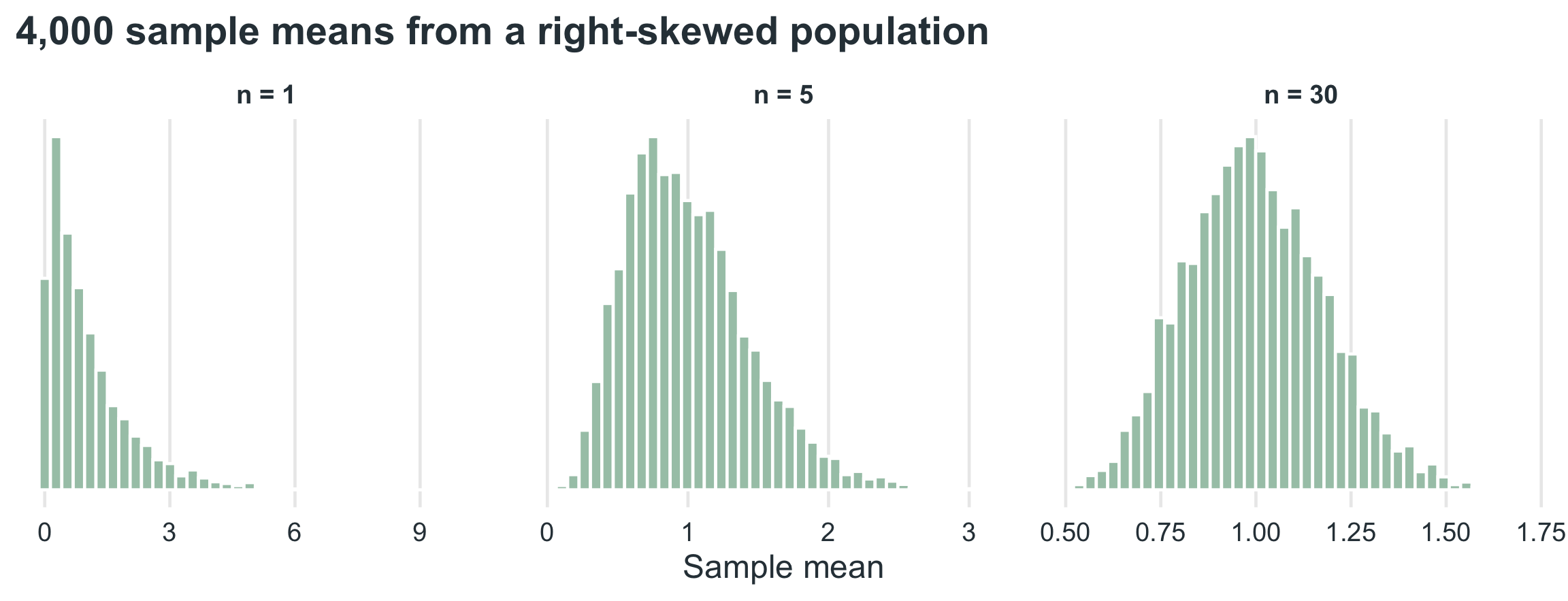
For large enough samples, the sampling distribution of the mean is approximately normal, centered at \(\mu\) with standard deviation \(\sigma / \sqrt{n}\), even when the population itself is not normal.

Central Limit Theorem

A skewed population, bell-shaped sample means

Z-Test

A z-score for a sample mean

Convert to z first

One student’s sample of \(n = 500\) has \(M = 6.75\). If \(\mu = 6.6\) and \(\sigma = 1.5\), how unusual is a sample mean this high?

• \(SE = \dfrac{\sigma}{\sqrt{n}} = \dfrac{1.5}{\sqrt{500}} = 0.067\)
• \(z = \dfrac{M - \mu}{SE} = \dfrac{6.75 - 6.6}{0.067} = 2.24\)

Z-Test

\(P(M \geq 6.75)\): more than (\(z = 2.24\))

Excerpt of the z-table (area to the left of z)

z	.03	.04	.05
2.1	0.9834	0.9838	0.9842
2.2	0.9871	0.9875	0.9878
2.3	0.9901	0.9904	0.9906

• By Hand
• In R

• Find 2.2 on the left side of the table and the .04 column.

• The table gives the area to the left: \(.9875\).

• We want 6.75 or more, so subtract from 1.

Reveal Answer

• \(1 - .9875 = .0125\)
• About 1.3% of samples of 500 would have a mean this high if \(\mu = 6.6\).

pnorm.R

# pnorm(q) = area to the LEFT of q; lower.tail = FALSE = area to the RIGHT (p-value)
# sd here is the standard error: sigma / sqrt(n)
1 - pnorm(2.24)                                          # .0125 (z-table)
pnorm(6.75, mean = 6.6, sd = 1.5 / sqrt(500),
      lower.tail = FALSE)                                # .0127 (unrounded z)

Example

Let me get uhh…

We want to know how much people like pizza.

• There are 12,500 people in our population. Each of the 25 of us collects a sample of 500.

• \(500 \times 25 = 12{,}500\)

• Each of us calculates the mean response from our sample of 500 people.

• What do we call those means?

  • What would it look like if we were to plot them?

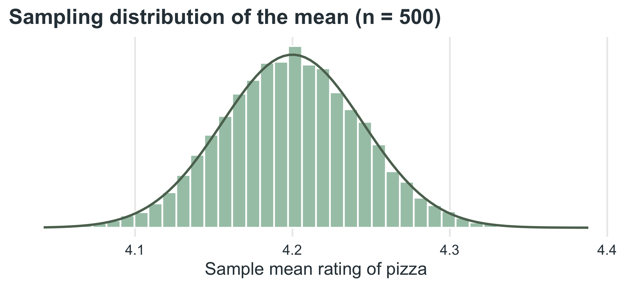
Pizza Plot

Visual example

Example

Pizza: a low sample mean

• I randomly choose one mean from our distribution of sample means about how much people like pizza.

• What is the probability of picking a mean with a z-score of -1 or less?

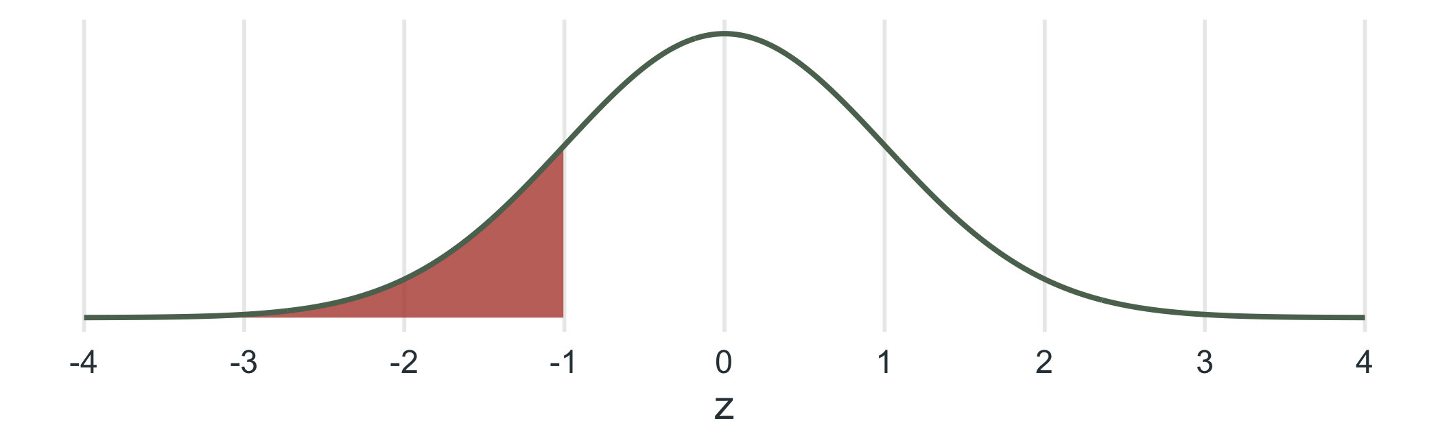
• \(P(z \leq -1) = .1587\), about 15.9%. The table gives the left area directly.

Sampling Theory

The big idea

Sampling theory is the body of principles that tells us how statistics from samples behave, so that we can make inferences about the population the samples came from.

• Take every possible sample of size \(n\) from a population and compute the mean of each. Those means form the sampling distribution of the mean.

• It is conceptual and theoretical. We never actually collect every possible sample.

Sampling Theory

What it buys us

• The sampling distribution of the mean is centered on \(\mu\), has standard deviation \(SE = \sigma / \sqrt{n}\), and is approximately normal for large \(n\).

• That lets us find the probability of getting a particular sample mean.

• We will use that probability to gauge significance in our inferential statistics.

Sampling Theory

With candy!

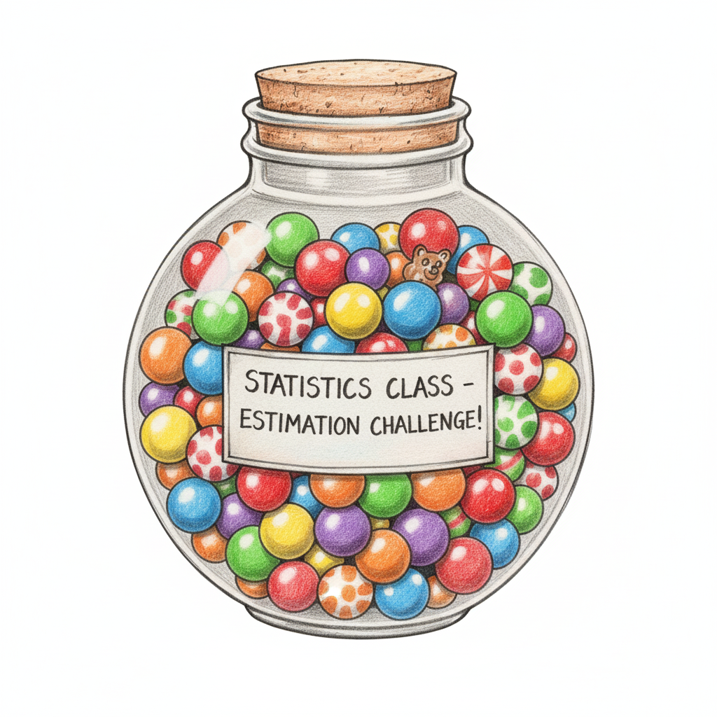
• This is a jar of 500 pieces of candy with 5 equally common flavors, so 100 are orange.

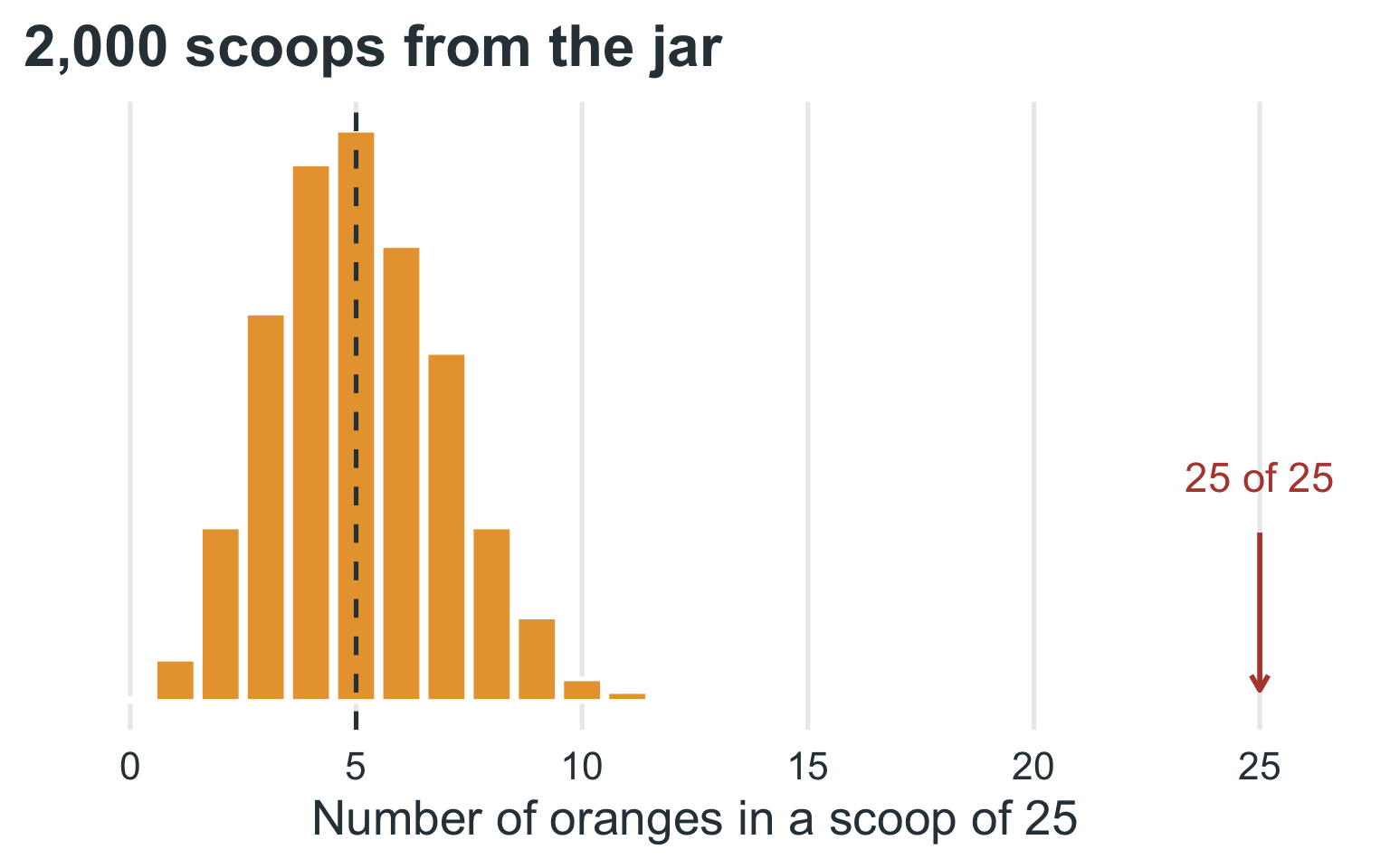
• If I took scoops of 25 pieces at a time, how many oranges should I expect per scoop?

  • \(25 \times \frac{100}{500} = 5\)

• I take a first scoop and 5 are orange. Is that surprising?

Sampling Theory

With candy!

• Is it safe to assume a 5-orange scoop came from the candy jar?

  • Probably!

• I take a scoop of 25 pieces and all 25 are orange.

• Did this scoop come from the candy jar?

  • Probably not

Null Hypothesis Significance Testing

NHST

A hypothesis is a testable prediction of what will happen in our experiment that:

• Names the variables (independent and dependent)

• Clearly contrasts the groups

NHST

Null and alternative hypotheses

Null Hypothesis \(H_0\)

• Nothing will happen: no difference between the groups.
• Names the variables (independent and dependent).
• \(\mu_1 = \mu_2\)

Alternative Hypothesis \(H_1/H_A\)

• A testable prediction that contrasts the groups.
• Names the variables (independent and dependent).
• \(\mu_1 > \mu_2\) (directional) or \(\mu_1 \neq \mu_2\) (non-directional)

NHST

Where the rejection region lives

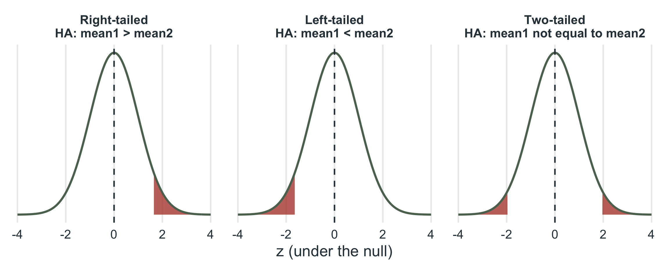
In every case \(H_0: \mu_1 = \mu_2\). The shaded rejection region holds the most extreme 5% of sample outcomes under the null (\(\alpha = .05\)): z beyond \(\pm 1.645\) in one tail, or beyond \(\pm 1.96\) split across two.

The Question

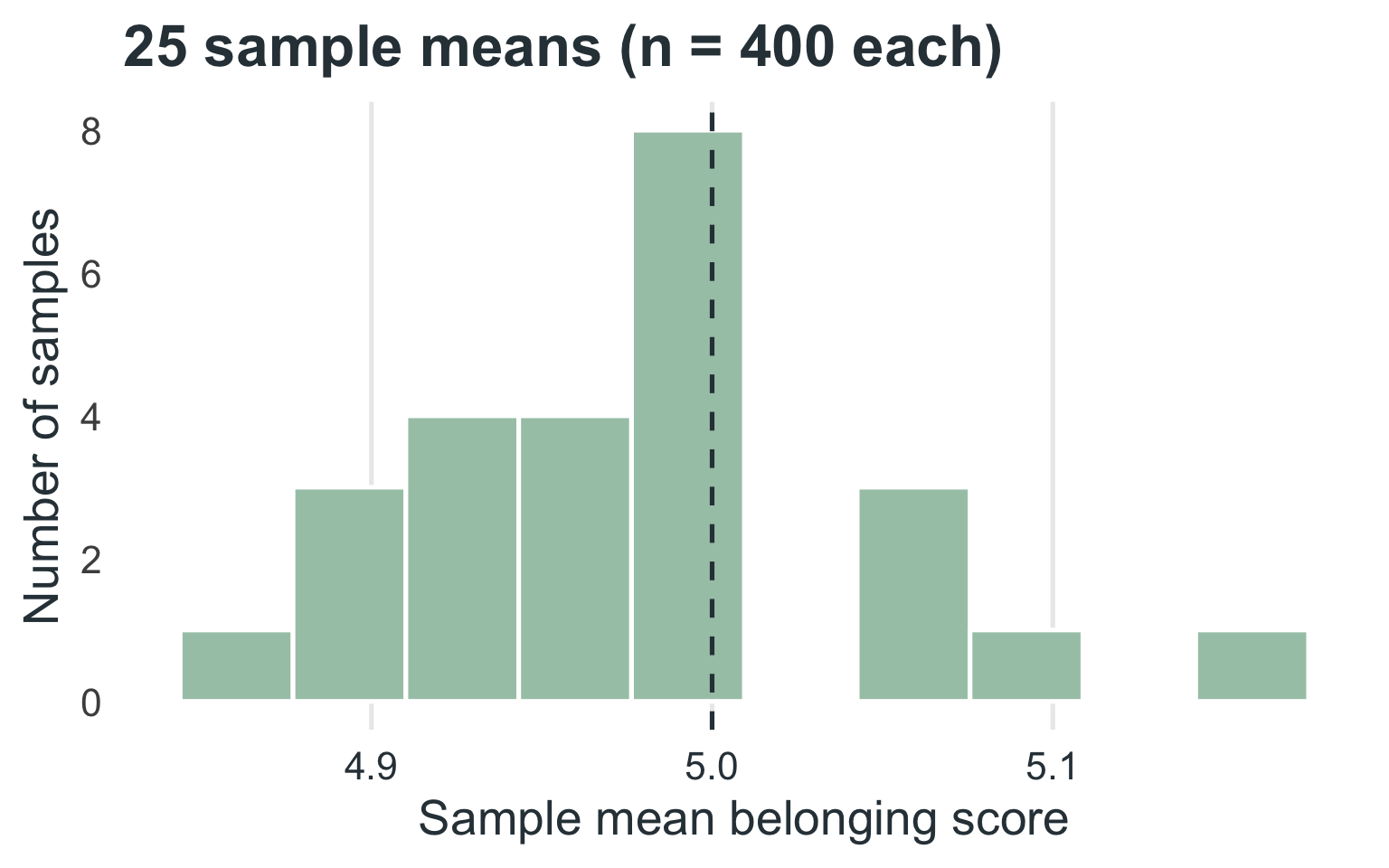
Every year we run a huge campus climate survey. We can’t ask all 10,000 students, so we draw a sample. Now imagine each of you is in charge of your own survey, each collecting 400 students’ responses.

• FSC has 10,000 students.

• Asking all 10,000 is not practical.

• Each of the 25 of us collects a sample of 400 students.

• We calculate the average belonging score in each sample.

  • These averages are called sample means.

Sampling Variation

• Sample means will not be identical.

• Why?

  • Different mixes of students (e.g., commuters, first-years, club leaders).

• This variation from sample to sample is called sampling variation.

  • It is the foundation of sampling theory.

Sampling Distribution

Campus survey

• If we plot all 25 sample means from FSC:

  • Most cluster near the true population mean (the dashed line).

  • Some fall higher or lower by chance.

• With more samples, this plot approaches the sampling distribution of the mean.

• With larger samples (bigger \(n\)), the sampling distribution becomes narrower.

Comparing Two Schools

We want to compare FSC students’ sense of belonging to that at another college. We draw 25 samples of 400 at each school.

• We repeat the study at John Jacob Jinglehymer Smith University (JJJSMU).

• We now have two sampling distributions:

  • One for FSC

  • One for JJJSMU

Comparing Two Schools

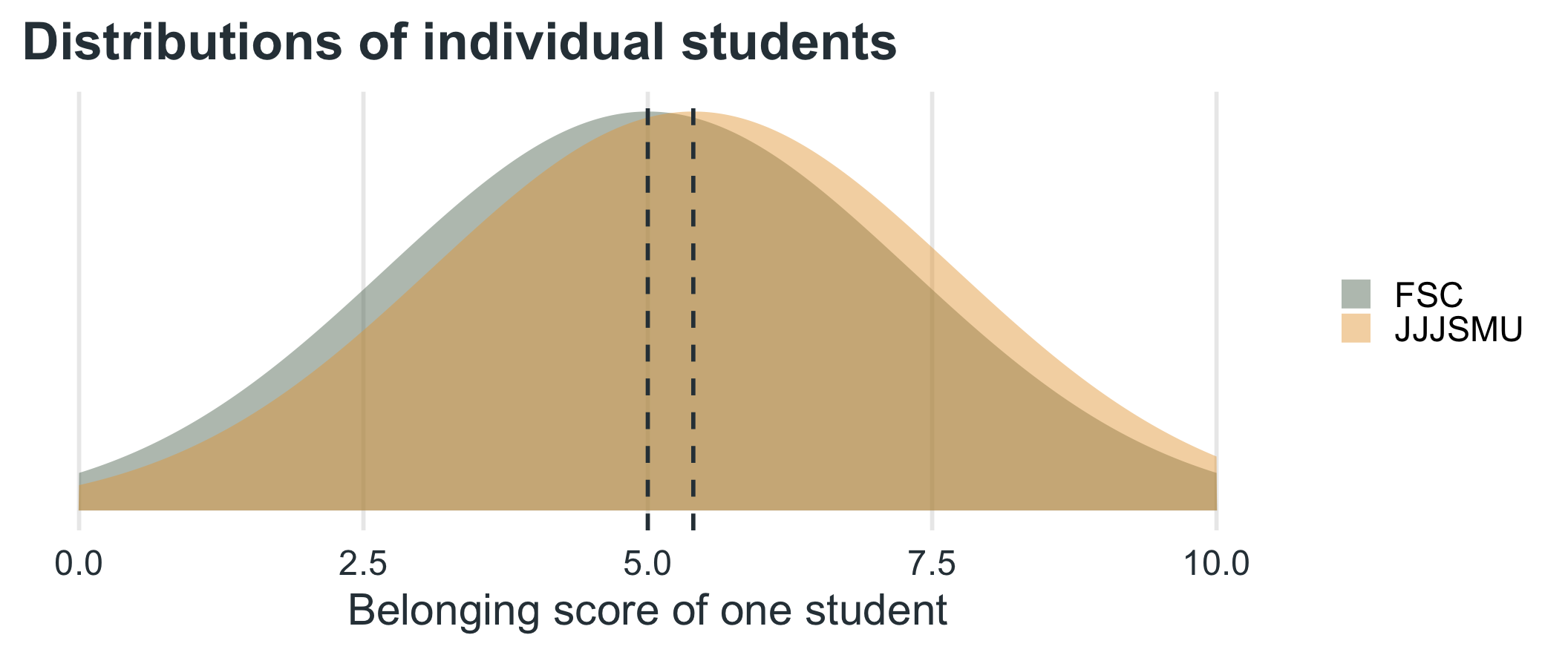
Individual students overlap a lot

Comparing Two Schools

Sample means separate

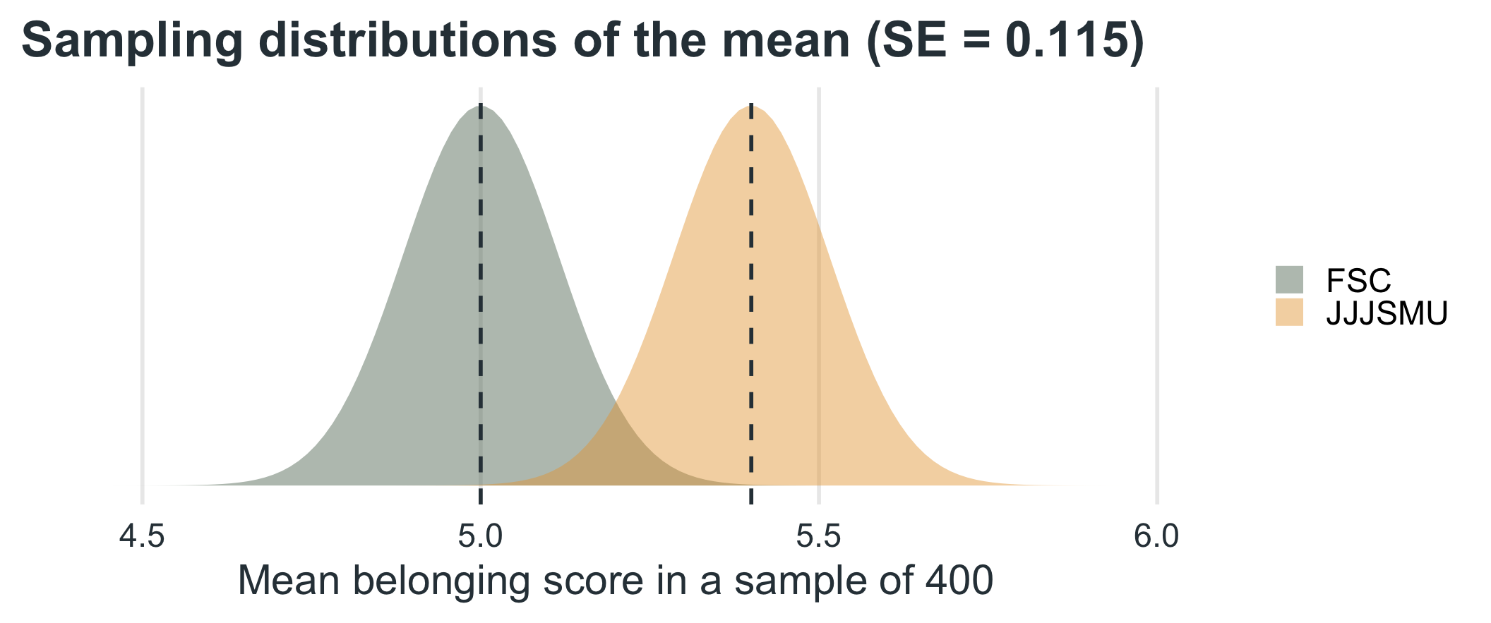
Same two schools, same data. The individual distributions overlap heavily. The sampling distributions of the mean overlap far less, because \(SE = \sigma/\sqrt{n}\) is much smaller than \(\sigma\).

Why It Matters

Sampling distributions let us:

• Estimate population parameters.

  • What is the population mean likely to be?

• Quantify sampling error.

  • The standard error tells us how much a sample mean typically bounces around \(\mu\).

• Compare populations in a statistically rigorous way.

  • Is the difference between two sample means bigger than sampling error alone would produce?

Probability

A refresher

The Lady Tasting Tea

The story

A lady declares that by tasting a cup of tea made with milk she can discriminate whether the milk or the tea infusion was first added to the cup. We will consider the problem of designing an experiment by means of which this assertion can be tested. […] [It] consists in mixing eight cups of tea, four in one way and four in the other, and presenting them to the subject for judgment in a random order. The subject has been told in advance of that the test will consist, namely, that she will be asked to taste eight cups, that these shall be four of each kind […]. — Fisher, 1935.

The Lady Tasting Tea

The design

• A lady claimed she could tell whether milk or tea was poured first.

• Fisher designed an experiment:

  • 8 cups of tea
  • 4 poured milk-first, 4 tea-first
  • Randomized order

• The lady must classify each cup.

A classic example of hypothesis testing, based on R.A. Fisher’s 1935 design.

The Hypotheses

Lady tasting tea

Null hypothesis \(H_0\)

The lady has no special ability; she is just guessing.

Alternative hypothesis \(H_1/H_A\)

The lady can tell the difference.

• Key idea: we begin by assuming \(H_0\) is true.

• We only reject \(H_0\) if the data are too surprising under \(H_0\).

Possible Outcomes

How many cups does she classify correctly?

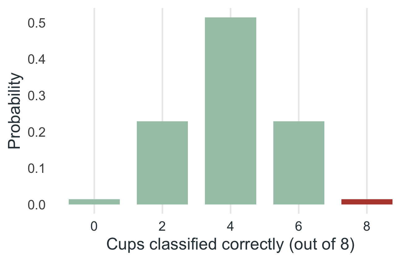
For 8 cups (4 of each), under \(H_0\) the number correct can only be 0, 2, 4, 6, or 8.

Correct	Probability
8	1 / 70 ≈ 1.4%
6	16 / 70 ≈ 22.9%
4	36 / 70 ≈ 51.4%
2	16 / 70 ≈ 22.9%
0	1 / 70 ≈ 1.4%

The Test

Fisher’s rule

• Reject \(H_0\) only if she gets all 8 correct.

• Under \(H_0\) there are \({8 \choose 4} = 70\) equally likely ways to guess which 4 cups are milk-first.

• So the probability of guessing all 8 correctly by chance is \(\dfrac{1}{70} \approx 1.4\%\).

Since \(1.4\%\) is less than \(5\%\), it is rare enough to count as evidence against \(H_0\).

Where the 70 Comes From

Choosing \(k\) items out of \(n\)

\[{n \choose k} = \dfrac{n!}{k!\,(n-k)!}\]

• \(n!\) (“n factorial”) means \(n \times (n-1) \times \dots \times 1\)
• The numerator, \(n!\), counts every ordering of all \(n\) items
• The denominator removes the orderings that do not matter: the order within the \(k\) chosen items, \(k!\), and within the \(n-k\) left out, \((n-k)!\)
• Here \(n = 8\) cups and \(k = 4\) milk-first: \(\dfrac{8!}{4!\,4!} = \dfrac{40{,}320}{24 \times 24} = 70\)

Decision & Interpretation

Lady tasting tea

8 of 8 correct: reject \(H_0\)

If she were just guessing, a result this extreme happens about 1.4% of the time. That is evidence she can tell the difference.

6 of 8 correct: fail to reject \(H_0\)

If she were just guessing, getting 6 or more right happens about \(\frac{1 + 16}{70} = 24.3\%\) of the time. That is not unusual enough.

We never prove the alternative; we only judge whether the data are too unlikely under the null.

The Logic

Same logic for t-tests, z-tests, and many modern methods

1. Assume a null model.
2. Compute how likely the observed data (or more extreme data) are under that model. That probability is the p-value.
3. If the p-value is very small (below \(\alpha\), typically .05), reject the null.

# k = how many of the 4 milk-first cups she correctly picks out (0-4)
# Correct cups out of 8 = 2k, so all 8 correct means k = 4
dhyper(0:4, m = 4, n = 4, k = 4)   # full distribution under H0

[1] 0.01428571 0.22857143 0.51428571 0.22857143 0.01428571

dhyper(4, m = 4, n = 4, k = 4)     # P(all 8 correct) = 1/70

[1] 0.01428571

Hypothesis

Example: Millennials and Gen Z

Professor Brocker wants to know if Millennials enjoy the Netflix Original Dark more than Gen Z does. He recruits 500 Millennials and 500 Gen Z students and asks them to rate Dark on a scale of 1 to 10 (10 being fantastic). Participants are not randomly assigned to generation, so this is a quasi-experiment.

• Hypothesis: Millennials will rate their enjoyment of Dark higher than their Gen Z peers.

Hypothesis

Example: Millennials and Gen Z

• Null hypothesis: the mean rating is the same for both generations.

  • \(H_0: \mu_{\text{Millennial}} = \mu_{\text{Gen Z}}\)

• Alternative hypothesis: the mean rating is higher for Millennials.

  • \(H_A: \mu_{\text{Millennial}} > \mu_{\text{Gen Z}}\)

Some texts write the null for a directional test as \(\mu_{\text{Millennial}} \leq \mu_{\text{Gen Z}}\). The decision rule is the same.

Hypothesis Testing

Example 1

Professor Brocker wants to know if giving his students coffee will improve their exam scores. He randomly assigns 13 of his 26 students to drink a doubleshot; he calls this the experimental group. The other 13 students drink decaf (a placebo); he calls this the control group.

• \(H_0\): \(\mu_\text{Coffee} = \mu_\text{Decaf}\)

• \(H_1/H_A\): \(\mu_\text{Coffee} > \mu_\text{Decaf}\)

Hypothesis Testing

Example 2

Esmeralda gives an anti-depressant to 100 individuals suffering from depression. She gives another 100 individuals a placebo. After 2 months, we measure their depression.

• \(H_0\): \(\mu_\text{SSRI} = \mu_\text{Placebo}\)

• \(H_1/H_A\): \(\mu_\text{SSRI} < \mu_\text{Placebo}\)

Hypothesis Testing

Practice

Jonas assigns half of the participants to engage in aerobic exercise for one hour a day for 6 months. The other half of the participants do not exercise for 6 months. At the end of the 6 months, Jonas measures the participants’ working memory capacity.

• \(H_0\): \(\mu_\text{Exercise} = \mu_\text{No Exercise}\)

• \(H_1/H_A\): \(\mu_\text{Exercise} > \mu_\text{No Exercise}\)

Decisions

Reject or fail to reject \(H_0\)

• In science, we do not say that we proved anything. Our decision is stated in terms of the null hypothesis \(H_0\).

• The decision depends on the p-value: the probability of getting data at least this extreme if \(H_0\) were true.

Reject \(H_0\) (\(p \leq \alpha\))

The data would be unlikely if \(H_0\) were true. The data are consistent with \(H_A\), but that is not a proof of \(H_A\).

Fail to reject \(H_0\) (\(p > \alpha\))

The data are not unlikely enough under \(H_0\). This is not evidence that \(H_0\) is true. A small sample or a noisy measure can hide a real effect.

Decisions

Neither outcome is a verdict on the study

• Rejecting \(H_0\) is the result we usually hope to see, but a well-run study that fails to reject is still informative.

• Failing to reject means “we did not find convincing evidence of a difference,” not “there is no difference.”

• When reporting a result, state the decision about \(H_0\) and give the test statistic and p-value.

Practice

Jonas

Jonas assigns half of the participants to engage in aerobic exercise for one hour a day, 5 days a week, for 6 months. The other half of the participants do not exercise for 6 months. At the end of the 6 months, Jonas measures the participants’ working memory capacity. His test is not significant.

• State Jonas’ findings in terms of the null hypothesis:

  • Jonas fails to reject the null hypothesis that there is no difference in working memory capacity between those who exercise and those who do not.

Practice

Brendan

Brendan assigns half of the participants to view a picture of a face on a mortuary table (control condition). The other half of the participants view an image of their own face made to look dead using a filter (experimental condition). Brendan then measures all participants’ anxiety about dying and runs a t-test, which is statistically significant.

• State Brendan’s findings in terms of the null hypothesis:

  • Brendan rejects the null hypothesis that there is no difference in death anxiety between participants who view their own face as deceased and those who view only a face on a mortuary table.