Standard Normal Distribution
PSY 348: Lecture 4
Dave Brocker
Farmingdale State College
Descriptive Statistics
The Old and the New
\(x\)
\(\bar{x}\)
\(\sum(x)\)
\(x^2\)
Descriptive Statistics
The Old and the New
\(x\) = refers to the value for 1 person (1 datapoint) in the sample
\(\bar{x}\) = refers to the mean or average value of X in the sample
\(\sum(x)\) = refers to the sum of all x values (sum of all the datapoints)
\(x^2\) = refers to the squared value of x (x multiplied by x)
Descriptive Statistics
Examples
\(data = \{1,4,3,2,4,6\}\)
\(x\) = \(1 | 4 | 3 | 2 | 4 | 6\)
\(\bar{x}\) = \(3.33\bar{3}\)
\(\sum(x)\) = \(1 + 4 + 3 + 2 + 4 + 6 = 20\)
\(x^2\) = \(1 | 16 | 9 | 4 | 16 | 36\)
Descriptive Statistics
Describe the characteristics of a sample in terms of:
Central tendency
The mid-point of the data
The most typical/frequent answers
Dispersion (aka Variability aka Variance)
- Dispersion: the action or process of distributing things or people over a wide area.
Central tendency: Mean
What is it, when should we use it, and how do we calculate it?
- Mean
- Average of all \(x\) values
- Normal Distribution
- Formula: \(\frac{\sum(x)}{n}\)
Central tendency: Median
What is it, when should we use it, and how do we calculate it?
- Median
- Middle value in sorted data
- Skewed distributions
- Is the data pulled to the left or the right?
- \(Med(X) = \frac{n + 1}{2}\)
Central tendency: Mode
What is it, when should we use it, and how do we calculate it?
- Mode
- Most common value
- Bi/Tri-Modal Distributions
- Most common value(s)
- Shows us that data is clustered
Central Tendency
What do measures of Central Tendency tell you?
The mid-point in the data
The answer most of the participants gave.
Central Tendency
What do measures of Central Tendency tell you?
Measures of Dispersion
What does dispersion mean?
Spread-out-ness
How much the participants’ responses differ from one another
Variance
Measures of Dispersion
Tells us about the spread-out-ness of the data, but what does that actually mean?
Measures of Dispersion
Measures of dispersion tell us about the spread-out-ness of the data, but what does that actually mean?
- If I am measuring phone usage what would low dispersion tell me?
- If I am measuring phone usage, what would high dispersion tell me?
Measures of Dispersion
Measures of dispersion tell us about consensus.
Did participants give similar answers?
- \(\{1,2,2,1,2,2,3,2,1\}\)
Did participants give wildly different answers?
- \(\{1,3,4,5,8,9,21,33\}\)
Dispersion
Measures of dispersion tell us about consensus.
Data should have natural dispersion.
If everyone gives a similar answer, it’s harder to analyze difference.
Calculating Dispersion
How do you think we should calculate dispersion?
On average, how far is each x-value from the midpoint
Calculate how far each x-value is from the midpoint (mean)
Take the average of those distances.
Calculating Dispersion
How do you think we should calculate dispersion?
In psychology, the mid-point we use will be the mean
Calculating Dispersion
Acquire Data
| Participant | X |
|---|---|
| 1 | 1 |
| 2 | 3 |
| 3 | 2 |
| 4 | 2 |
| 5 | 3 |
| 6 | 2 |
| 7 | 1 |
| 8 | 3 |
| 9 | 1 |
| 10 | 2 |
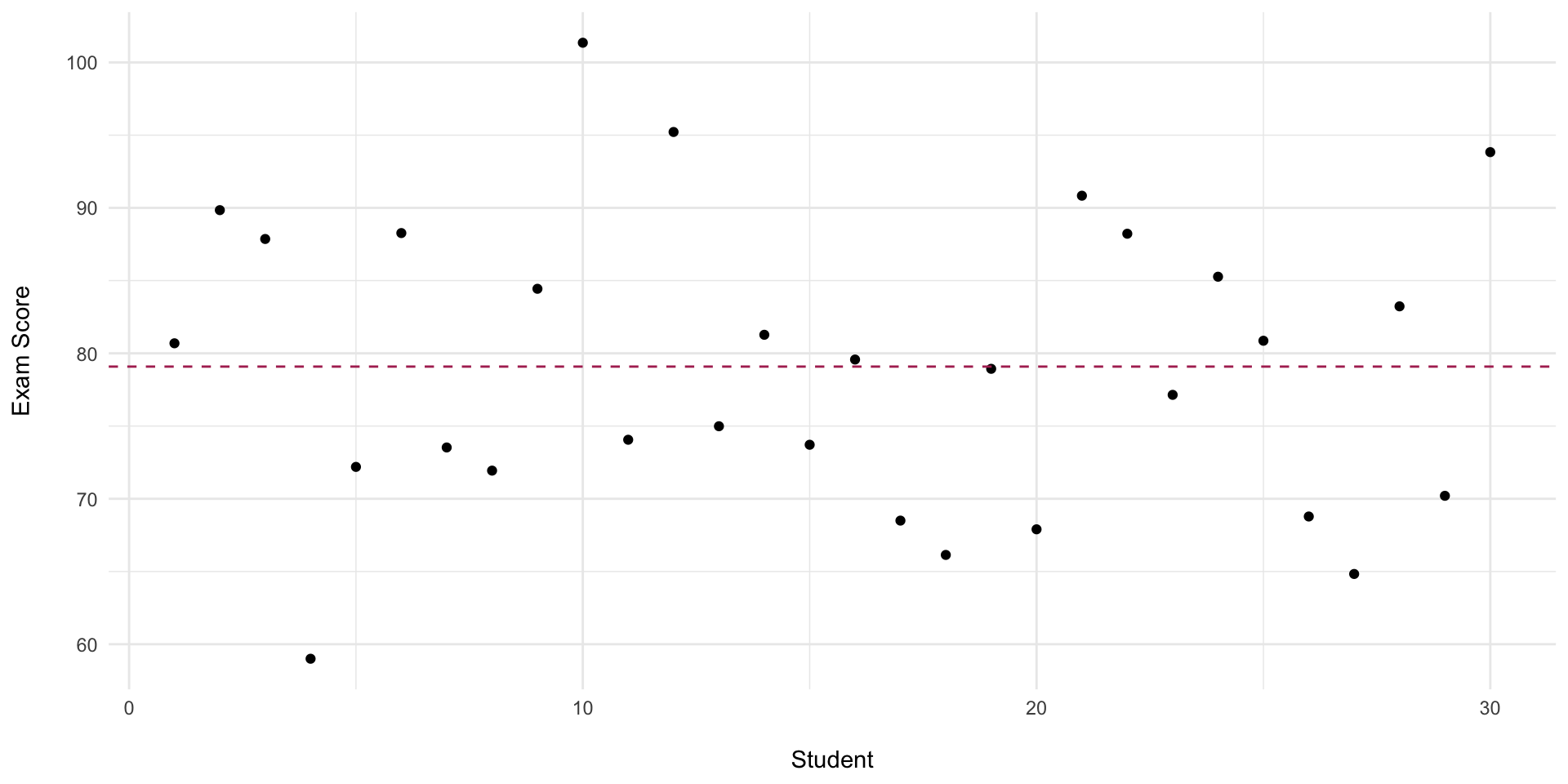
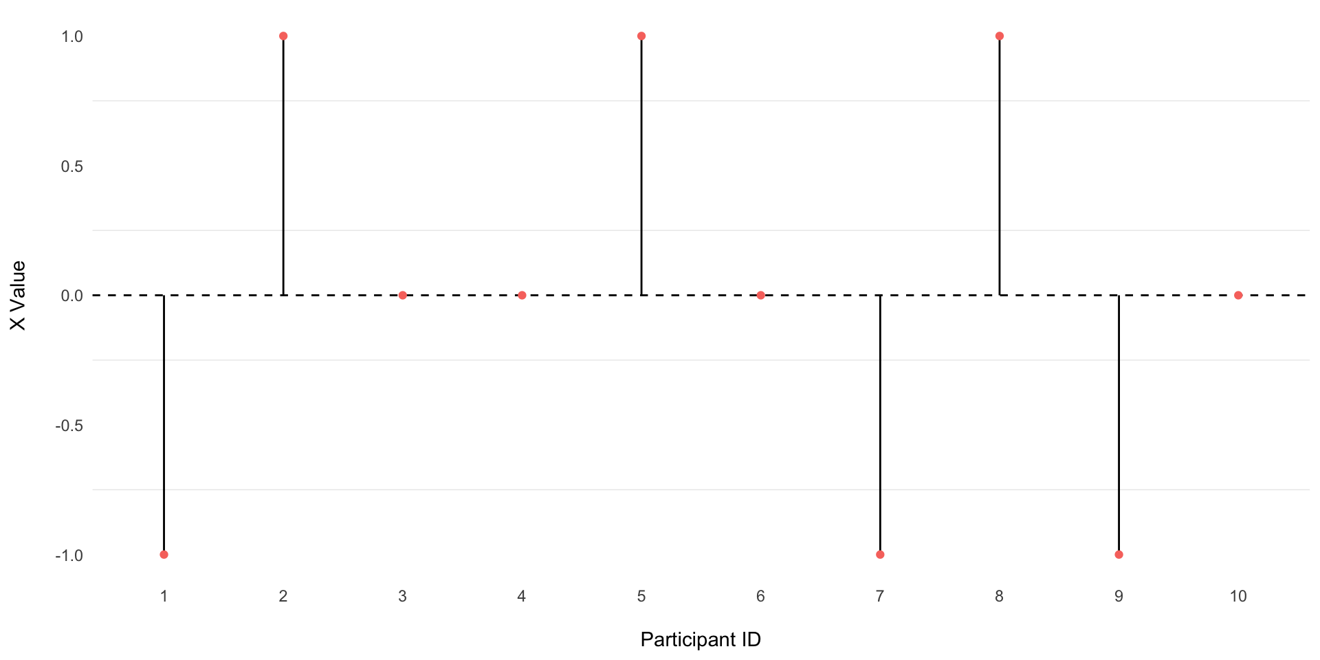
Deviation Scores
Calculate how far each x-value is from the mean
Step 1. Examine Data
- \(data = \{1,3,2,2,3,2,1,3,1,2\}\)
Step 2. Calculate Mean
\(\bar{x} = \frac{\sum(x)}{n} = 1 + 3 + 2...\)
\(\bar{x} = \frac{20}{10} = 2\)
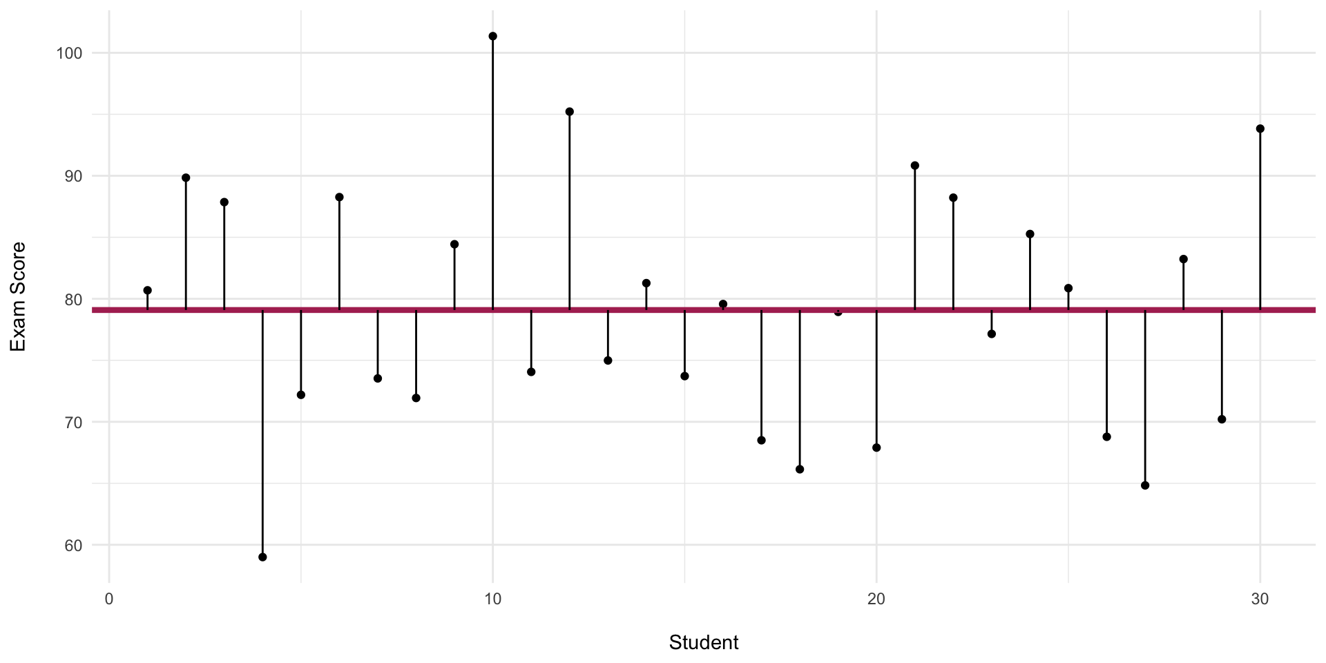
Deviation Scores
Calculate how far each x-value is from the mean
Step 2: Subtract the mean from each X-value.
\(x - \bar{x}\)
\((1-2) + (3-2) + (2-2) + (2-2)...\)
\((-1) + 1 + 0 + 0...\)
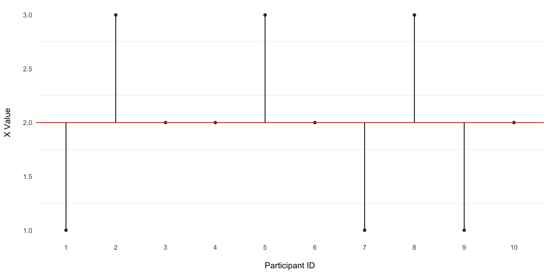
Calculating Dispersion
Visual
| ParticipantID | x | \(x-\bar{x}\) |
|---|---|---|
| 1 | 1 | -1 |
| 2 | 3 | 1 |
| 3 | 2 | 0 |
| 4 | 2 | 0 |
| 5 | 3 | 1 |
| 6 | 2 | 0 |
| 7 | 1 | -1 |
| 8 | 3 | 1 |
| 9 | 1 | -1 |
| 10 | 2 | 0 |
Calculating Dispersion
Visual
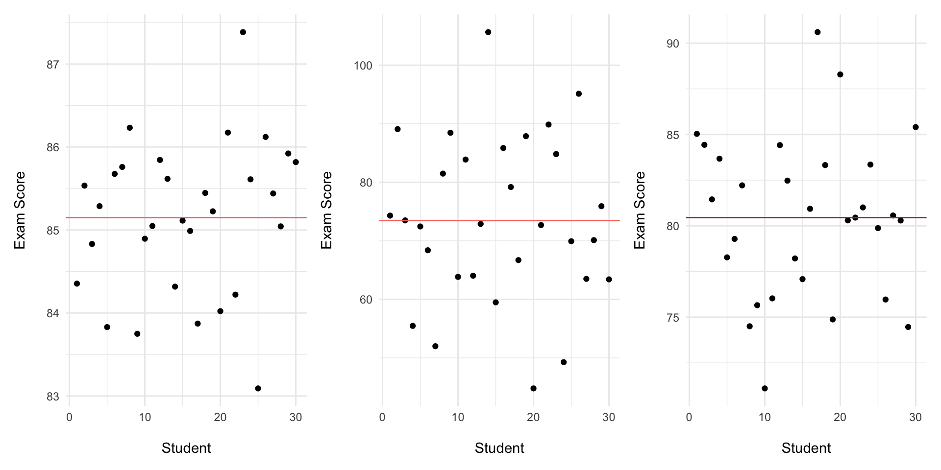
Calculating Dispersion
Visual
Calculating Dispersion
Visual
The average of the deviation scores will always = 0.
On average, the x-values = x.
So the average distance of x from x is 0.
Calculating Dispersion
How do you think we should calculate dispersion?
- Calculate the mean.
- Calculate the deviation scores.
- What can we do to the deviation scores to prevent them from adding up to 0?
What is the Mean of the Deviation Scores?
Stop Being So Negative!
The problem is the negative numbers!
How do we get rid of negative numbers
\((x-\bar{x})^2 = (1-2) = 0 | (1-2)^2 = 1\)
Calculating Dispersion
Stop Being So Negative!
| ParticipantID | x | \((x-\bar{x})\) | \((x-\bar{x}^2)\) |
|---|---|---|---|
| 1 | 1 | -1 | 1 |
| 2 | 3 | 1 | 1 |
| 3 | 2 | 0 | 0 |
| 4 | 2 | 0 | 0 |
| 5 | 3 | 1 | 1 |
| 6 | 2 | 0 | 0 |
| 7 | 1 | -1 | 1 |
| 8 | 3 | 1 | 1 |
| 9 | 1 | -1 | 1 |
| 10 | 2 | 0 | 0 |
Calculating Dispersion
First 3 Steps
Step 1: Calculate the mean.
Step 2: Subtract the mean from each X-value.
Step 3: Square each deviation score.
Calculating Dispersion
Now what: Calculate the average squared deviation.
Step 4: Add up the Squared Deviations.
\(1+1+0+1...\)
Calculating Dispersion
Now what: Calculate the average squared deviation.
| ParticipantID | x | \((x-\bar{x})\) | \((x-\bar{x}^2)\) |
|---|---|---|---|
| 1 | 1 | -1 | 1 |
| 2 | 3 | 1 | 1 |
| 3 | 2 | 0 | 0 |
| 4 | 2 | 0 | 0 |
| 5 | 3 | 1 | 1 |
| 6 | 2 | 0 | 0 |
| 7 | 1 | -1 | 1 |
| 8 | 3 | 1 | 1 |
| 9 | 1 | -1 | 1 |
| 10 | 2 | 0 | 0 |
Calculating Dispersion
Divide by n-1 to Estimate
Step 5: Divide by (n-1).
(n-1) refers to the degrees of freedom… don’t worry about it for now.
\(\frac{\sum (x-\bar{x})^2}{n-1}\)
Variance
- The fact or quality of being different, divergent, or inconsistent.
Calculating Dispersion
How do think we should calculate dispersion?
When we squared the deviation scores in Step 3, we inflated the deviation.
We have to undo that inflation.
How do you undo squaring?
We take the square root.
Calculating Dispersion
Inflation
| ParticipantID | X | \((x-\bar{x})\) | \((x-\bar{x}^2)\) | |
|---|---|---|---|---|
| 1 | 40.55 | −2.79 | 7.782 | |
| 2 | 48.55 | 5.21 | 27.145 | |
| 3 | 46.751 | 3.411 | 11.636 | |
| 4 | 42.035 | −1.304 | 1.701 | |
| 5 | 45.682 | 2.342 | 5.485 | |
| 6 | 36.47 | −6.869 | 47.188 | |
| Sum | — | — | — | 100.93818 |
| Mean | — | — | — | 20.18764 |
Calculating Dispersion
Step 6: Take the square root.
- \(\sqrt{\frac{\sum(x-\bar{x})^2}{n-1}}\)
Calculating standard deviation
Step-by-Step
Mean: Calculate the mean.
- \(\bar{x}\)
Deviation scores: Subtract the mean from each x-value.
- \((x-\bar{x})\)
Squared deviations: Square each deviation score.
- \((x-\bar{x})^2\)
Sum of squares: Add up the squared deviations.
- \(\sum(x-\bar{x})^2\)
Calculating standard deviation
Step-by-Step
Variance: Divide the sum of squares by (n-1).
- \(\frac{\sum(x-\bar{x})^2}{n-1}\)
Standard Deviation: Take the square root of the variance.
- \(\sqrt{\frac{\sum(x-\bar{x})^2}{n-1}}\)
Formulas for Dispersion
Variance and Standard Deviation
Variance
\[ \large{\color{gold}{s^2} = \frac{\sum(x-\bar{x})^2}{n-1}} \]
Standard Deviation
\[ \large{\color{orange}{s} = \sqrt{\frac{\sum(x-\bar{x})^2}{n-1}}} \]
Formulas for Dispersion
Standard Deviation
Variance is a measure of dispersion.
- It’s not helpful, because it’s inflated (from squaring the deviation scores).
Standard deviation is a better measure of dispersion, because it is standardized.
- This means that a standard deviation of 1 means a distance of 1 on the scale used to measure x.
Variance & Standard deviation
The Variance is the standard deviation squared: s²
The Standard Deviation is the square root of the variance: s
Practice 1 — Basic mean, deviations, variance, SD
Problem (do by hand first):
Compute the sample mean, each deviation from the mean, the sum of squared deviations, the sample variance, and the sample standard deviation for the dataset:
x = [4, 2, 5, 6, 3]
Practice 1
Solution (steps)
- Sum: \((\sum x = 4+2+5+6+3 = 20)\)
- Sample size: \((n = 5)\)
- Mean: \((\bar{x} = \frac{20}{5} = 4)\)
- Deviations: \((x_i - \bar{x} = [0, -2, 1, 2, -1])\)
- Squared deviations: \(([0, 4, 1, 4, 1])\)
- Sum of squared deviations: \((0+4+1+4+1 = 10)\)
- Sample variance: \((s^2 = \frac{\sum (x_i-\bar{x})^2}{n-1} = \frac{10}{4} = 2.5)\)
- Sample SD: \((s = \sqrt{2.5} \approx 1.5811)\)
x <- c(4,2,5,6,3)
n <- length(x)
sum_x <- sum(x)
mean_x <- mean(x)
deviations <- x - mean_x
sq_dev <- deviations^2
ssd <- sum(sq_dev)
s2 <- var(x)  # sample variance by default (n-1)
s <- sd(x)
list(
  n = n,
  sum = sum_x,
  mean = mean_x,
  deviations = deviations,
  squared_deviations = sq_dev,
  sum_squared_deviations = ssd,
  sample_variance = s2,
  sample_sd = s
)
$n
[1] 5
$sum
[1] 20
$mean
[1] 4
$deviations
[1] 0 -2 1 2 -1
$squared_deviations
[1] 0 4 1 4 1
$sum_squared_deviations
[1] 10
$sample_variance
[1] 2.5
$sample_sd
[1] 1.581139Problem 2: Comparing dispersion
Mathematically
Two instructors have class scores: - Class A: scores_A = \([80, 82, 78, 85, 75]\) - Class B: scores_B = \([60, 90, 75, 85, 85]\) 1. Compute the mean and sample SD for each class. 2. Both classes have similar means. Which class has greater dispersion? What does that imply about reporting a “typical” student score?
Problem 2: Comparing dispersion
Mathematically
Step 1: Compute the mean
- \(\bar{x}_A = \frac{80+82+78+85+75}{5} = \frac{400}{5} = 80\)
Step 2: Compute deviations and squared deviations
\(x_i - \bar{x}_A = [0, 2, -2, 5, -5]\)
\((x_i - \bar{x}_A)^2 = [0, 4, 4, 25, 25]\)
Step 3: Compute variance and SD
\(s_A^2 = \frac{\sum (x_i - \bar{x}_A)^2}{n-1} = \frac{58}{4} = 14.5\)
\(s_A = \sqrt{14.5} \approx 3.81\)
Step 1: Compute the mean
- \(\bar{x}_B = \frac{60+90+75+85+85}{5} = \frac{395}{5} = 79\)
Step 2: Compute deviations and squared deviations
\(x_i - \bar{x}_B = [-19, 11, -4, 6, 6]\)
\((x_i - \bar{x}_B)^2 = [361, 121, 16, 36, 36]\)
Step 3: Compute variance and SD
\(s_B^2 = \frac{\sum (x_i - \bar{x}_B)^2}{n-1} = \frac{570}{4} = 142.5\)
\(s_B = \sqrt{142.5} \approx 11.94\)
Interpretation
- Class A: \(\bar{x} = 80, s \approx 3.81\)
- Class B: \(\bar{x} = 79, s \approx 11.94)\)
Problem 2: Comparing dispersion
Computationally
Dispersion | ⬡⬢⬡⬢