bar_chart scatter_plot show_chart pie_chart table_chart insert_chart

Data Visualization

PSY 348: Lecture 2

Dave Brocker
brockeda@farmingdale.edu
Farmingdale State College

From “Stats Is Everywhere” to “Let’s Actually See It”

Last time: statistics isn’t just math — it’s how you make sense of decisions you already make every day.

smartphone

• A number by itself is hard to feel — “the average score was 78” doesn’t tell you much on its own

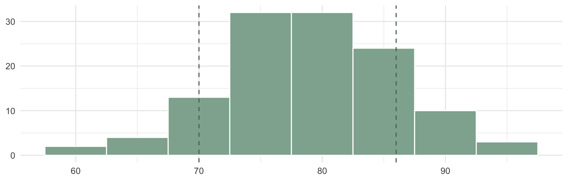
The average was 78. You scored a 67.

Today: choosing and building the right picture for your data.

Why Visualize Data?

Consider these two ways of showing the same information:

Option A

78

(SD = 8)

Option B

Both are “true.” Only one of them lets you see the students who didn’t fit the average.

Same Numbers, Very Different Pictures

Anscombe’s Quartet

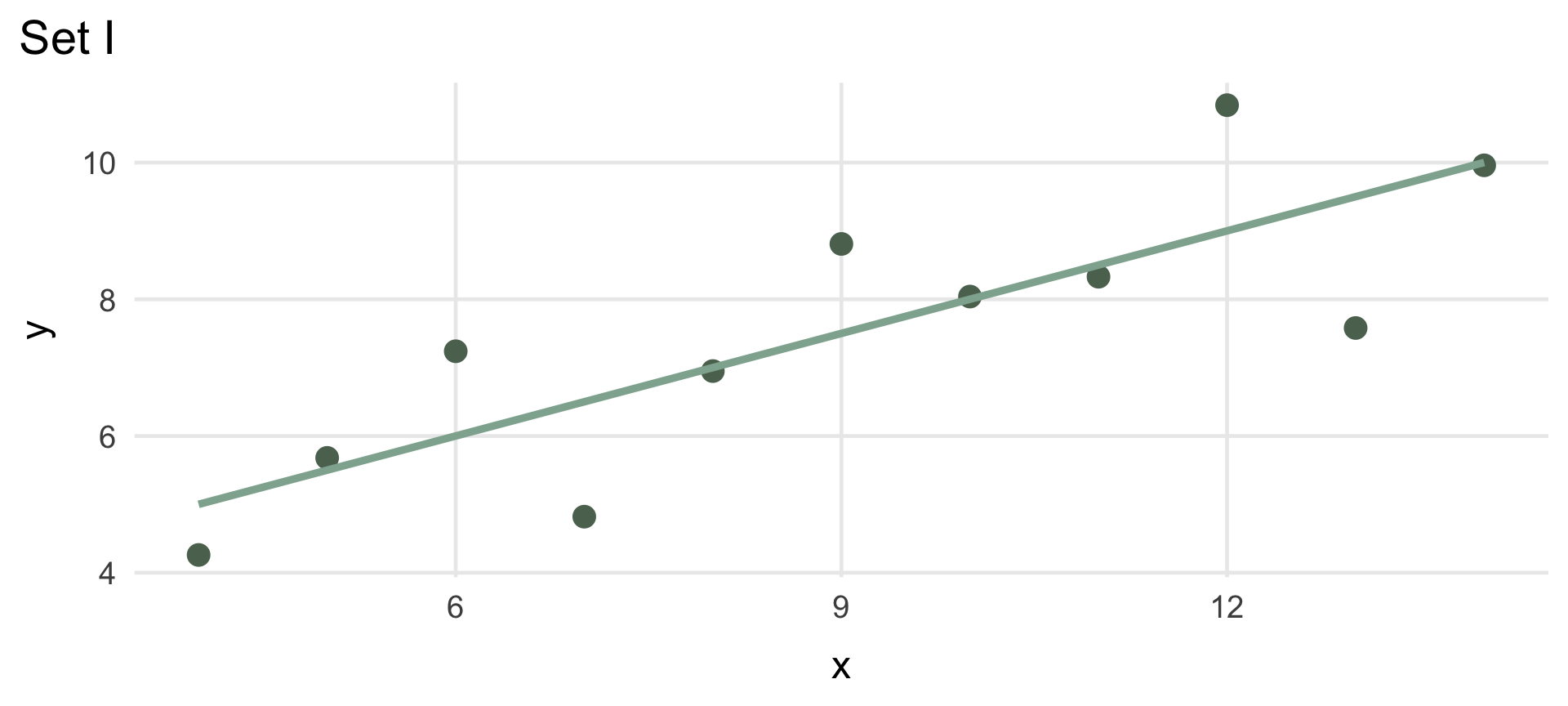
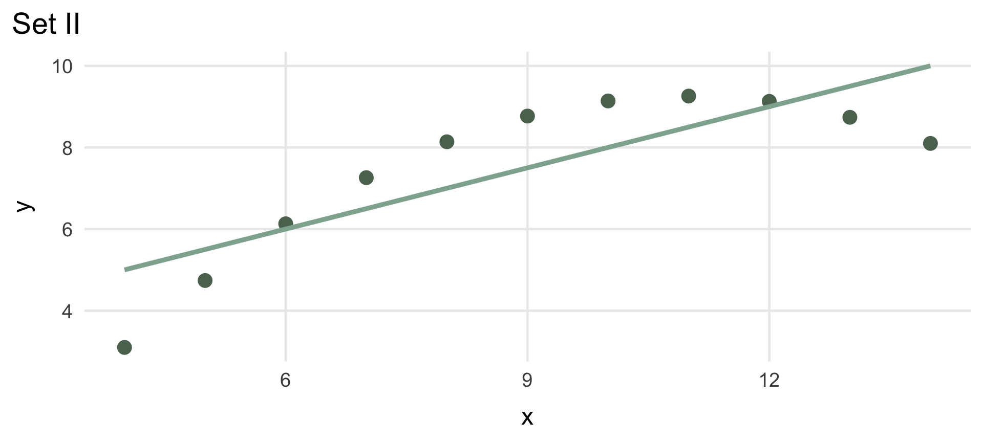
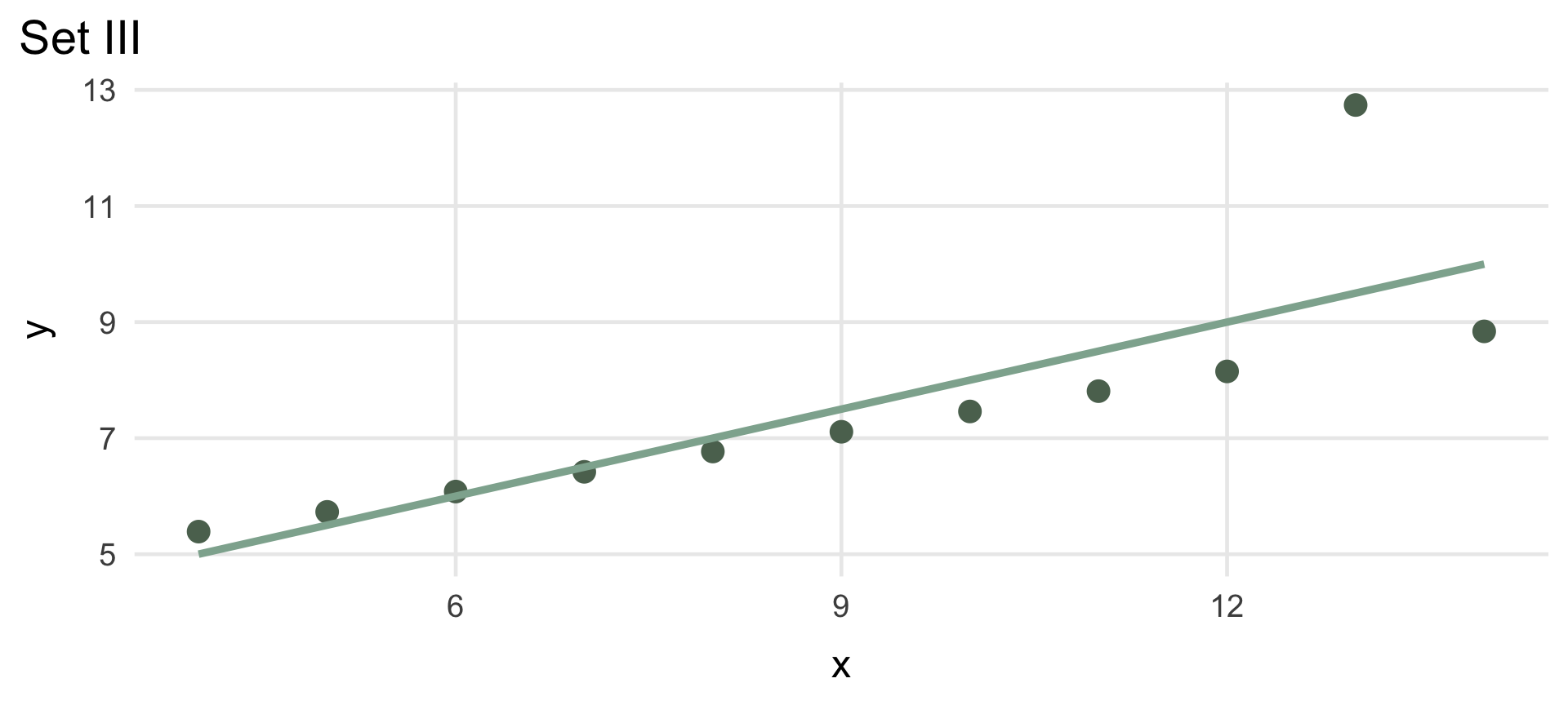
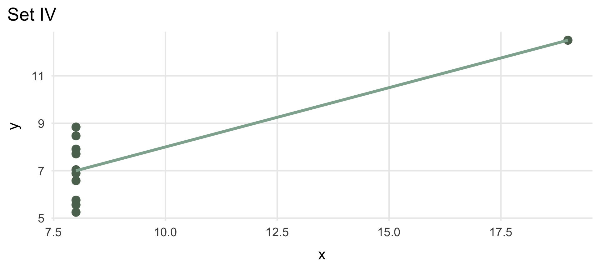
These four datasets have (essentially) identical descriptive statistics:

Anscombe's Quartet: Identical Summary Statistics
	Mean (x)	Mean (y)	SD (x)	SD (y)	Correlation
I	9	7.5	3.32	2.03	0.82
II	9	7.5	3.32	2.03	0.82
III	9	7.5	3.32	2.03	0.82
IV	9	7.5	3.32	2.03	0.82
Anscombe, F. J. (1973). Graphs in statistical analysis.

Same Numbers, Very Different Pictures

But Look What They Actually Look Like

• Set I
• Set II
• Set III
• Set IV

Same mean, SD, and correlation in every tab — click through them. Four very different pictures.

The Takeaway

• Summary statistics (mean, SD, correlation) can hide the actual shape of your data

• Outliers, clusters, and non-linear patterns are often invisible in a table of numbers

• Always look at the picture — it’s not optional, it’s part of the analysis

Choosing the Right Chart

A Quick Decision Guide
	What are you showing?	Best chart
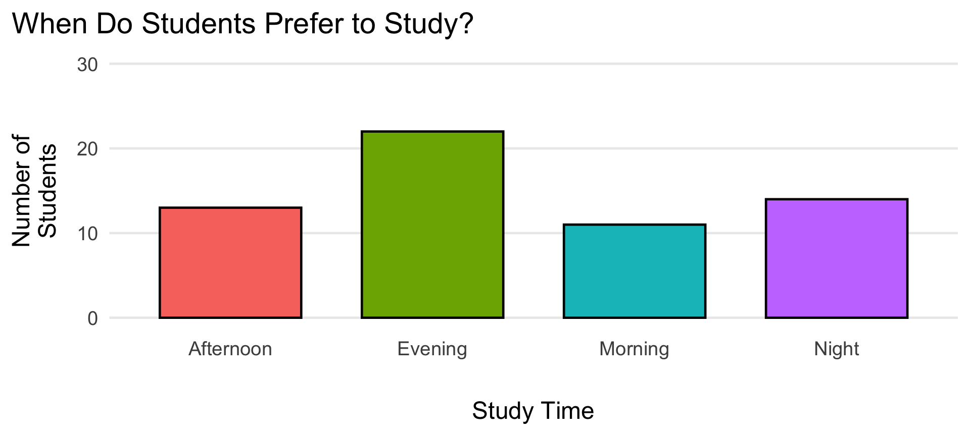
bar_chart	One categorical variable (counts per group)	Bar chart
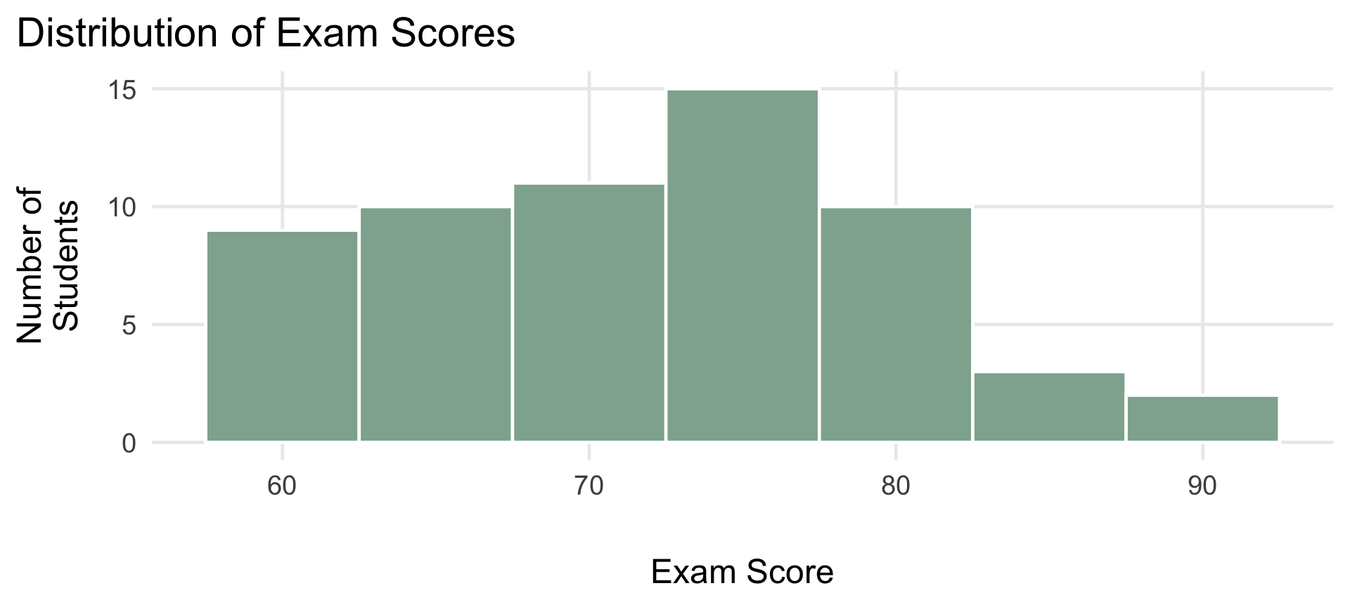
insert_chart	One continuous variable (its shape/spread)	Histogram or density plot
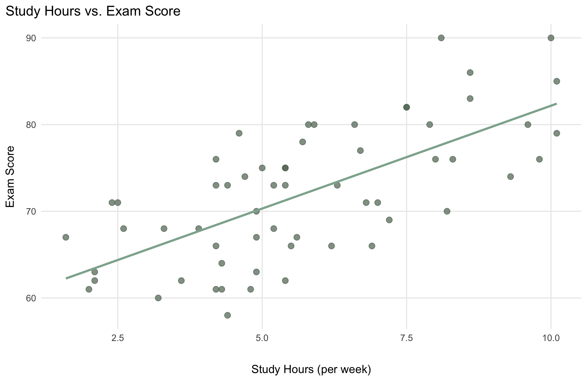
scatter_plot	Two continuous variables (a relationship)	Scatterplot
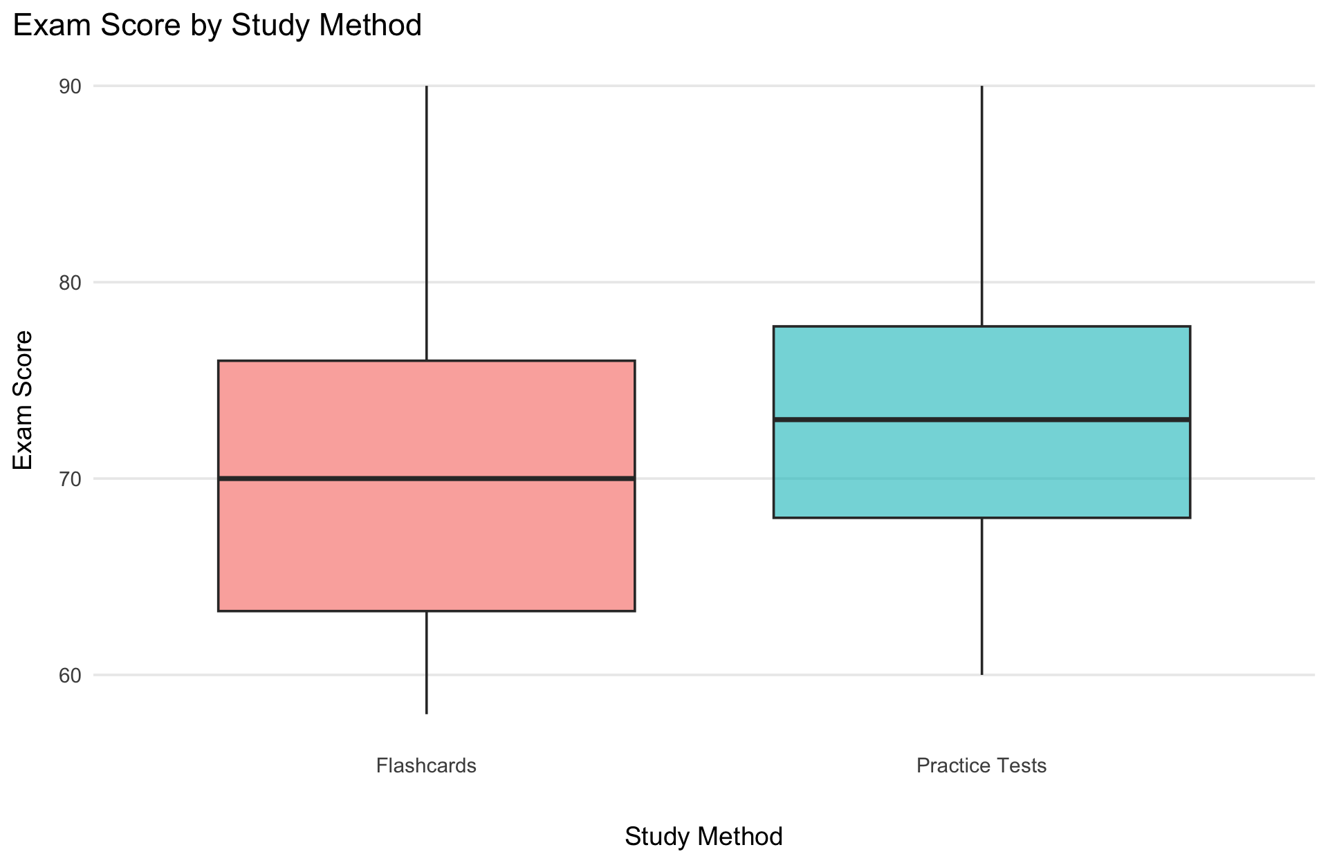
equalizer	A continuous variable, compared across groups	Box plot
show_chart	Change over time	Line chart

The ggplot2 Recipe

Every ggplot2 chart follows the same three-ingredient recipe — we’ll come back to this constantly this semester. It’s ggplot2’s implementation of Wilkinson’s “Grammar of Graphics”: any chart can be built from the same small set of parts.

table_chart

Data

Which tibble/data frame are you plotting?

tune

Aesthetics

aes() — which columns map to x, y, color, etc.?

bar_chart

Geometry

geom_*() — what shape represents your data?

ggplot(data, aes(x = ..., y = ...)) +
  geom_something()

1

Data + aesthetics — the data frame, and which columns map to x/y/color/etc.

2

Geometry — the shape (bars, points, lines…) that represents your mapped data.

We’ll build up from this simple recipe all semester — no need to memorize every option today.

Example Student Data

One Dataset, Several Questions

set.seed(2)  # makes the "random" data reproducible every time this renders
students <- tibble(
  student = 1:60,                                             # just an ID number
  study_time = sample(c("Morning", "Afternoon", "Evening", "Night"), 60,
                       replace = TRUE, prob = c(0.15, 0.30, 0.35, 0.20)),   # categorical variable
  study_hours = pmax(round(rnorm(60, mean = 6, sd = 2), 1), 0.5),          # continuous variable, floor at 0.5
  study_method = rep(c("Flashcards", "Practice Tests"), each = 30),       # two even groups
  exam_score = pmin(round(55 + 2.5 * study_hours +                        # score rises with study hours...
                     ifelse(study_method == "Practice Tests", 4, 0) +     # ...gets a small bump from practice tests...
                     rnorm(60, 0, 5)), 100)                               # ...plus random noise, capped at 100
)

readr::write_csv(students, "students.csv")  # so it can be linked/downloaded below

students |>
  slice_head(n = 5) |>       # just preview the first 5 rows
  gt() |>
  tab_header(title = "Example Student Data") |>
  opt_row_striping() |>
  tab_options(table.font.size = 22, table.width = pct(80)) |>
  tab_style(style = cell_text(weight = "bold"), locations = cells_column_labels()) |>
  cols_align(align = "center", columns = everything())

Example Student Data
student	study_time	study_hours	study_method	exam_score
1	Evening	7.5	Flashcards	82
2	Night	6.6	Flashcards	80
3	Afternoon	8.2	Flashcards	70
4	Evening	5.4	Flashcards	62
5	Morning	4.4	Flashcards	58

⬇ Download students.csv

Bar Charts

One Categorical Variable

Histograms

One Continuous Variable

Scatterplots

Two Continuous Variables

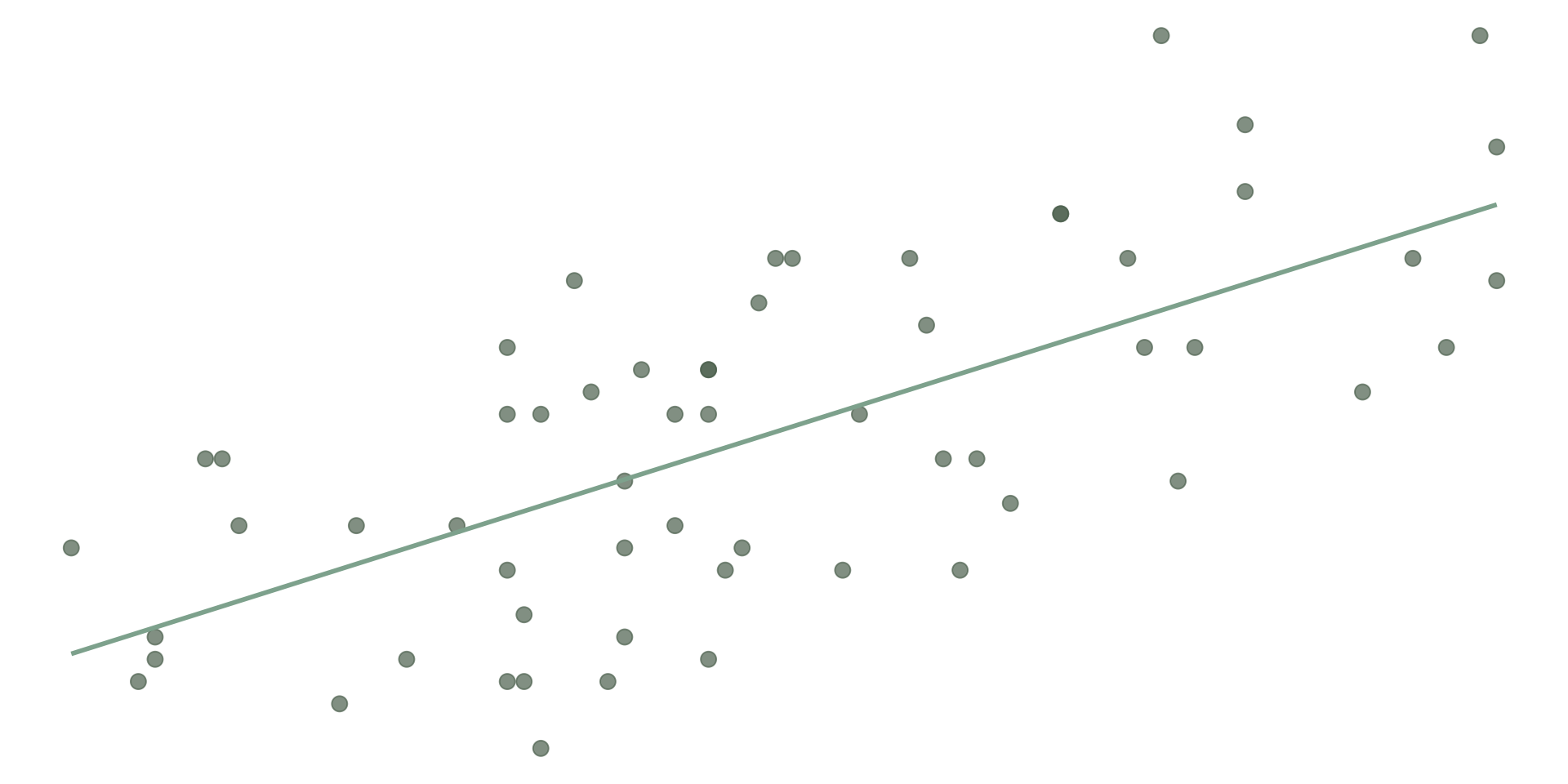
We’ll come back to this exact question — “how strongly are two variables related?” — when we get to correlation.

Box Plots

Comparing a Continuous Variable Across Groups

This is also a preview — “is the difference between these two groups big enough to matter?” is exactly what a later lecture’s t-test answers.

How Graphs Can Mislead

Same Data, Different Story

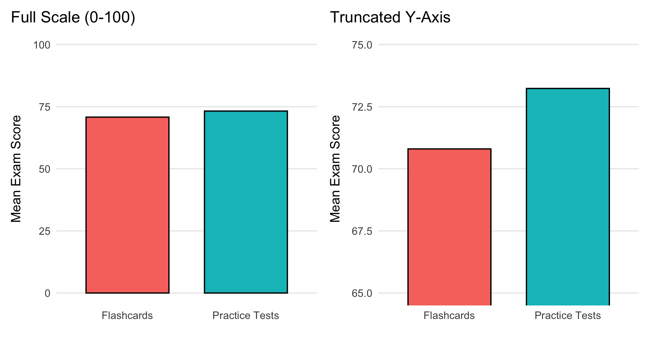
Same exact numbers. The right panel makes a small difference look dramatic — always check where the y-axis starts.

Building a Good Graph

• Title — what am I looking at?

• Labeled axes — with units, if relevant

• An honest scale — start bar charts at 0; don’t cherry-pick a range to exaggerate a difference

• Only the elements that add information — no 3D effects, no unnecessary gridlines, no clutter

Guess This Chart

Fill in the blank

What’s on the x-axis? The y-axis? What relationship is this showing — and what chart type is it?

Guess This Chart, Too

Fill in the blank

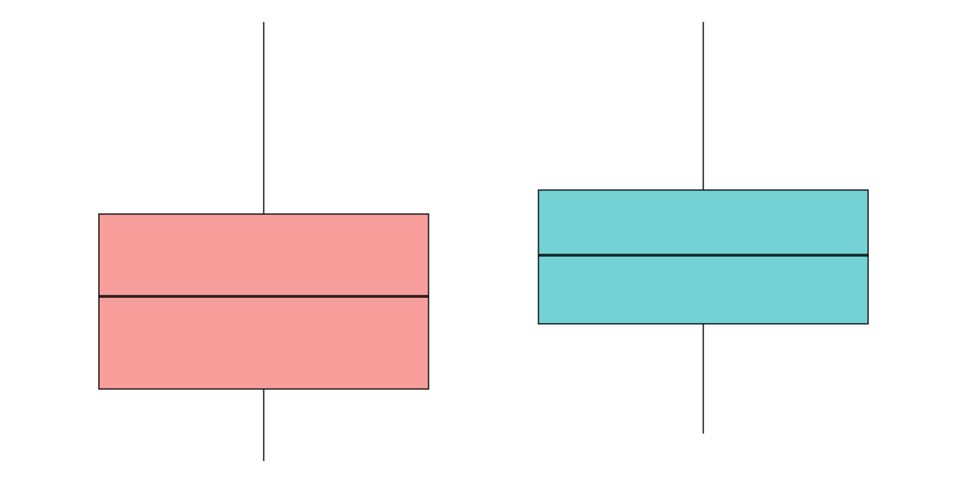
No axis labels this time either — what are the two groups probably being compared, and what does the shape of each box tell you?

Recap: What You Should Walk Away With

• A summary statistic can hide the actual shape of your data — that’s why we plot it

• You can match a research question to the right chart: one variable vs. two, categorical vs. continuous, one group vs. several

• You’ve seen the basic ggplot2 recipe: data + aesthetics + geometry — the “Grammar of Graphics”

• You know how to spot (and avoid) a few common ways graphs mislead

Next time: back to describing that shape with numbers — measures of central tendency.