ANOVA (Analysis of Variance), like t-tests, compares the means of different groups to determine if they differ significantly from one another:
Independent variable: Categorical / Nominal
Dependent variable: Continuous
When to Use Repeated Measures ANOVA
Use Repeated Measures ANOVA when:
You have the same participants measured more than once (e.g., pre-test/post-test).
You’re interested in changes over time or under different conditions.
Example: Testing whether students’ enjoyment of statistics improves after receiving lollipops for 2 weeks.
Between vs. Within Subjects ANOVA
Between-Subjects ANOVA:
Compares means between groups (e.g., Group A vs. Group B).
Error comes from individual differences between people.
Within-Subjects (Repeated Measures) ANOVA:
Compares means within the same participants over time.
Controls for individual differences.
🍕 Pizza and Productivity Study
A Repeated-Measures Design
Objective: Test whether productivity changes across three timepoints:
Before lunch
10 minutes after pizza
1 hour after pizza
Same participants measured at each timepoint
DV = Number of emails written in 10 minutes
What type of test compares means across more than two repeated timepoints?
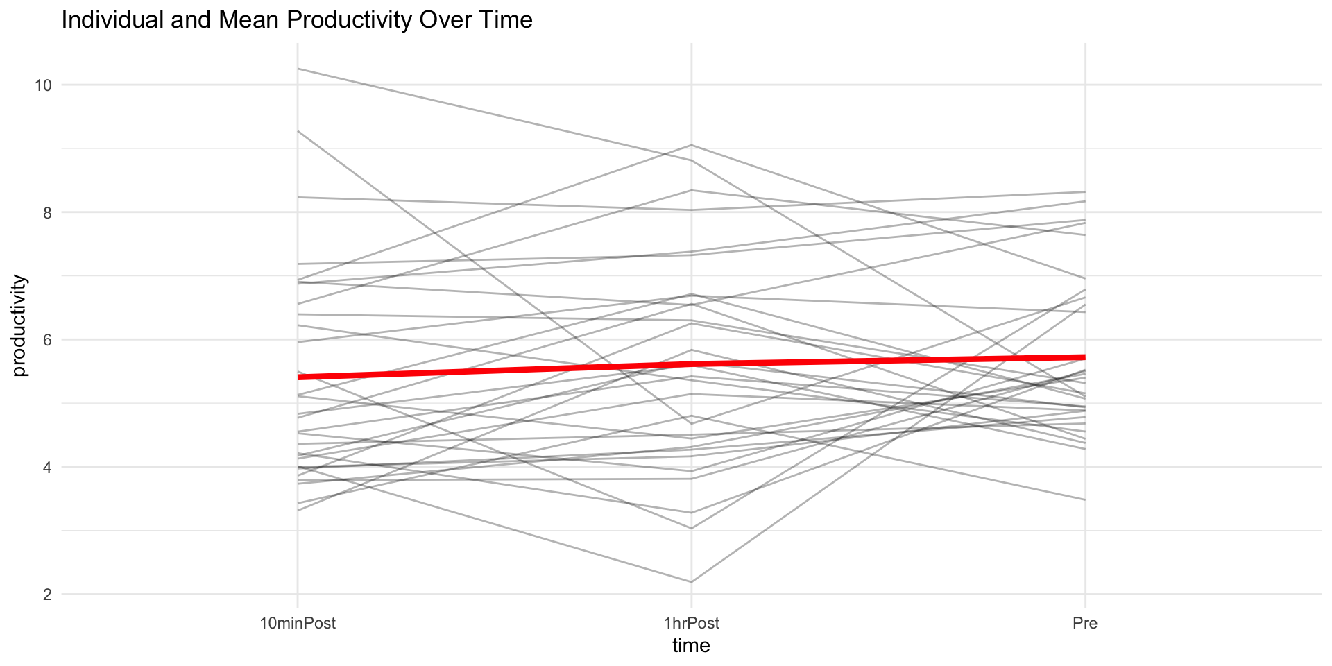
📊 Visualizing the Data
Code
library(tidyverse)set.seed(123)data <-tibble(id =rep(1:30, each =3),time =rep(c("Pre", "10minPost", "1hrPost"), times =30),productivity =c(rnorm(30, mean =5, sd =1),rnorm(30, mean =7, sd =1.5),rnorm(30, mean =4.5, sd =1) ))data %>%ggplot(aes(x = time, y = productivity, group = id)) +geom_line(alpha =0.3) +stat_summary(aes(group =1), fun = mean, geom ="line", color ="red", size =1.5) +labs(title ="Individual and Mean Productivity Over Time") +theme_minimal()
🧪 Why Repeated-Measures ANOVA?
Can’t use multiple paired-samples t-tests (increases Type I error)
Repeated-Measures ANOVA allows us to:
Compare within-subject changes across time
Control for individual variability
Test for an overall time effect
📐 Assumptions of RM ANOVA
Normality of differences
Sphericity: Equal variances of pairwise differences
Test: Mauchly’s Test
Violation → Use Greenhouse-Geisser correction
Always check sphericity if more than two levels of the within-subject factor
🧮 Running the Analysis in R
✅ Interpretation
Example output:
F(2, 58) = 12.3, p < .001
→ Significant effect of time on productivity
Conclusion: Productivity changes significantly across timepoints
What would be your next step?
🔍 Follow-Up: Post-hoc Comparisons
Run paired t-tests with Bonferroni correction
Which timepoints differ?
Pre vs. 10minPost
10minPost vs. 1hrPost
Pre vs. 1hrPost
ANOVA
Between subjects ANOVA compares means BETWEEN groups to determine if they differ significantly from one another.
Within subjects ANOVA compares pre-manipulation means to post-manipulation means to determine if there is a difference WITHIN participants over time.
Within subjects ANOVA
Within subjects ANOVA examines differences within participants over time.
Within subjects ANOVA is also known as Repeated Measures ANOVA, because it looks at one measure repeated over time.
Within subjects ANOVA
The independent variable is time.
Before intervention: baseline or pre-test
After intervention: post-test
Within Subjects ANOVA
Within subjects ANOVA can look at 2 or more time points.
WITHIN Subjects ANOVA
Code
library(ggplot2)library(dplyr)library(gt)library(gtsummary)library(broom)library(afex)# Generate data for two normal distributionsx <-seq(-6, 6, length=100)null_dist <-dnorm(x, mean =0, sd =1)alt_dist <-dnorm(x, mean =2, sd =1)data <-data.frame(x =rep(x, 2),y =c(null_dist, alt_dist),hypothesis =factor(rep(c("Null Hypothesis", "Alternative Hypothesis"), each=length(x))))# Create the plotplt <-ggplot(data, aes(x = x, y = y, lty =rev(hypothesis))) +geom_line(aes(color ="purple")) +theme_linedraw() +labs(x ="",y ="",lty ="Hypotheses" ) +theme(panel.grid =element_blank(),legend.position ="inside",legend.position.inside =c(.2,.5),legend.background =element_rect(color ="black") ) +scale_color_identity()plt
Between subjects ANOVA
In between subjects ANOVA, we analyze two types of variance:
Between Group variance: How the data varies between the groups
Error variance: How the data varies across all participants
Between subjects ANOVA
Between Group variance: How the data varies between the groups
Error variance: How the data varies across all participants
WITHIN subjects ANOVA
In within subjects ANOVA the variance is more complicated, because data will differ in 3 ways:
Over time
Error variance: How the data varies across all participants
Per participant
WITHIN subjects ANOVA Example
In within subjects ANOVA the variance is more complicated, because data will differ in 3 ways:
Over time: Mood before Dark is more similar to mood before Dark than it is to mood after the Dark
WITHIN subjects ANOVA
WITHIN subjects ANOVA Example
In within subjects ANOVA the variance is more complicated, because data will differ in 3 ways:
Over time: Mood before the Dark is more similar to mood before Dark than it is to mood after the Dark
Error Variance: Mood will have natural variance across participants and time.
WITHIN subjects ANOVA Example
WITHIN subjects ANOVA Example
In within subjects ANOVA the variance is more complicated, because data will differ in 3 ways:
Over time: Mood before Dark is more similar to mood before Dark than it is to mood after Dark
Error Variance: Mood will have natural variance across participants.
Per participant: Each participant’s scores will be more like their other scores than they are like the scores of another participant.
WITHIN subjects ANOVA Example
WITHIN subjects ANOVA
In within subjects ANOVA the variance is more complicated, because data will differ in 3 ways:
Time
Error
Subjects
WITHIN subjects ANOVA
Code
flowchart LR
      A(Total Variability) --> B(Time Variability)
      A --> C(Within-Groups Variability)
      C --> D(Subject Variability)
      C --> E(Error Variability)
flowchart LR
      A(Total Variability) --> B(Time Variability)
      A --> C(Within-Groups Variability)
      C --> D(Subject Variability)
      C --> E(Error Variability)
Calculating F
WITHIN subjects ANOVA
What is the F ratio in between subjects ANOVA?
\(F = \frac{MS_{BG}}{MS_{Error}}\)
WITHIN subjects ANOVA
What is the F ratio in between subjects ANOVA?
\(F = \frac{\color{red}{MS_{BG}}}{MS_{Error}}\)
\(MS_{BG} = \frac{SS_{BG}}{df_{BG}}\)
WITHIN subjects ANOVA
What is the F ratio in between subjects ANOVA?
\(F = \frac{MS_{BG}}{\color{red}{MS_{Error}}}\)
\(MS_{Error} = \frac{SS_{Error}}{df_{Error}}\)
WITHIN subjects ANOVA
We want measure 2 sources of variance:
\(SS_{Time}\): this is just like the SS from between subjects ANOVA
\(SS_{Error}\): this is harder to calculate in within subjects ANOVA, because of the subject variance.
Prof. Brocker wants to know if giving lollipops to statistics students improves their opinion of statistics. He asks 100 students to rate how much they enjoy statistics on a scale of 1 (not at all) to 10 (extremely). Then he gives each student a lollipop at the start of statistics class for 2 weeks. After two weeks of conditioning, Prof. Brocker asks participants to rate how much they enjoy statistics again.
What’s k?
What’s n?
Practice
Prof. Brocker wants to know if giving lollipops to statistics students improves their opinion of statistics. He asks 100 students to rate how much they enjoy statistics on a scale of 1 (not at all) to 10 (extremely). Then he gives each student a lollipop at the start of statistics class for 2 weeks. After two weeks of conditioning, Prof. Brocker asks participants to rate how much they enjoy statistics again.
Prof. Brocker wants to know if giving lollipops to statistics students improves their opinion of statistics. He asks 100 students to rate how much they enjoy statistics on a scale of 1 (not at all) to 10 (extremely). Then he gives each student a lollipop at the start of statistics class for 2 weeks. After two weeks of conditioning, Prof. Brocker asks participants to rate how much they enjoy statistics again.
Dr. Grace believes watching Shameless makes Zoomers happy. She asks 50 Zoomers to rate their happiness on a scale of 1 (no happies) to 10 (all the happies). Then she shows them an episode of Shameless. After each Zoomer watches one episode of Shameless, she asks them to rate their happiness again on the same scale of 1 to 10.
What’s k?
What’s n?
Practice
ANOVA
Prof. Brocker measures the death anxiety of 500 middle-aged men. He then shows them images from anti-aging advertisements featuring young men. After they view the images, participants report their aging anxiety once again. Two weeks later, participants are asked to report their aging anxiety one last time.
What’s k?
What’s n?
Practice
Interpreting f
The MSTime is made up of the MSError + the theoretical difference over time:
\(MS_{Time} = \text{change over time} + MS_{Error}\)
\(MS_{Time} = 0 + MS_{Error}\)
\(MS_{Time} = MS_{Error}\)
\(F = 1\)
Interpreting f
When F <= 1, it’s not likely to be significant.
Interpreting f
The MSTime is made up of the MSError + the theoretical difference over time:
\(MS_{Time} = \text{change over time} + MS_{Error}\)
\(MS_{Time} = \text{effect} + MS_{Error}\)
\(F > 1\)
Hypothesis testing: ANOVA
F < = 1 —> Fail to reject the Null Hypothesis
F > 1 —> Refer to p-value —> Reject the Null Hypothesis
How many F’s do you Get?
One-way Between Subjects?
1 for 1 IV
Two-way Between Subjects with a 2x2 design?
3 (One for each IV and one for the Interaction)
Within Subjects?
1
Reporting F
Reporting F
If asked to report findings in terms of the Null Hypothesis (H0), you should report findings as:
Reject H0, or
Fail to Reject H0
Reporting F
If asked to report findings in general or for publication, you need to report:
F(df time, df error) = F-value, p-value
Reporting F
Mood after watching the Dark was not significantly different from mood before watching Dark, F (1, 499) = 1.02, p = 0.07.
There was no significant change in mood over time, F (1, 499) = 1.02, p = 0.07.
Reporting F
Participants’ mood was significantly better after watching the Dark compared to before watching it, F(1, 499) = 7.12, p < 0.05.
Reporting F
If asked to report findings in general or for publication, you need to report:
F(df time, df error) = F-value, p-value
If the results are significant, we have to also report the means and standard deviations for each time point.
Reporting F
Participants’ anxiety differed significant across time, F(2, 198) = 3.744, p = 0.25. Anxiety was highest at pre-test (M= 19.58, s = 0.643). Anxiety was lowest at baseline (M , s ). Anxiety at post test was M= , s.
Practice
Was anxiety just before the Stats Exam significantly higher than baseline anxiety?
Data Manipulation
When collected, data can be in either wide or long format.
Below are the first five rows of the same dataset:
Code
data.frame(Participant =factor(1:5),Immediate =rnorm(5, mean =8, sd =1.5),After24Hours =rnorm(5, mean =6, sd =1.5),After1Week =rnorm(5, mean =4, sd =1.5)) |>gt() |>tab_header(title ="Wide Data",subtitle ="Each row represents an indivdual participant")
Wide Data
Each row represents an indivdual participant
Participant
Immediate
After24Hours
After1Week
1
7.629962
3.498087
1.573176
2
7.478686
5.429660
3.916657
3
6.572572
7.378495
4.779111
4
7.932458
5.136980
4.451730
5
6.822643
6.911946
4.158514
Code
data.frame(Participant =factor(1:5),Immediate =rnorm(5, mean =8, sd =1.5),Day =rnorm(5, mean =6, sd =1.5),Week =rnorm(5, mean =4, sd =1.5)) |> tidyr::pivot_longer(cols =!Participant,names_to ="Time",values_to ="Stress") |>gt() |>fmt_auto() |>tab_header(title ="Long Data",subtitle ="Each row represents an indivdual participant's score on each level of the treatment")
Long Data
Each row represents an indivdual participant's score on each level of the treatment
Participant
Time
Stress
1
Immediate
10.807
1
Day
5.637
1
Week
3.411
2
Immediate
8.904
2
Day
7.676
2
Week
4.011
3
Immediate
6.851
3
Day
7.777
3
Week
0.258
4
Immediate
7.07
4
Day
8.47
4
Week
2.534
5
Immediate
9.185
5
Day
6.289
5
Week
4.943
More Examples!
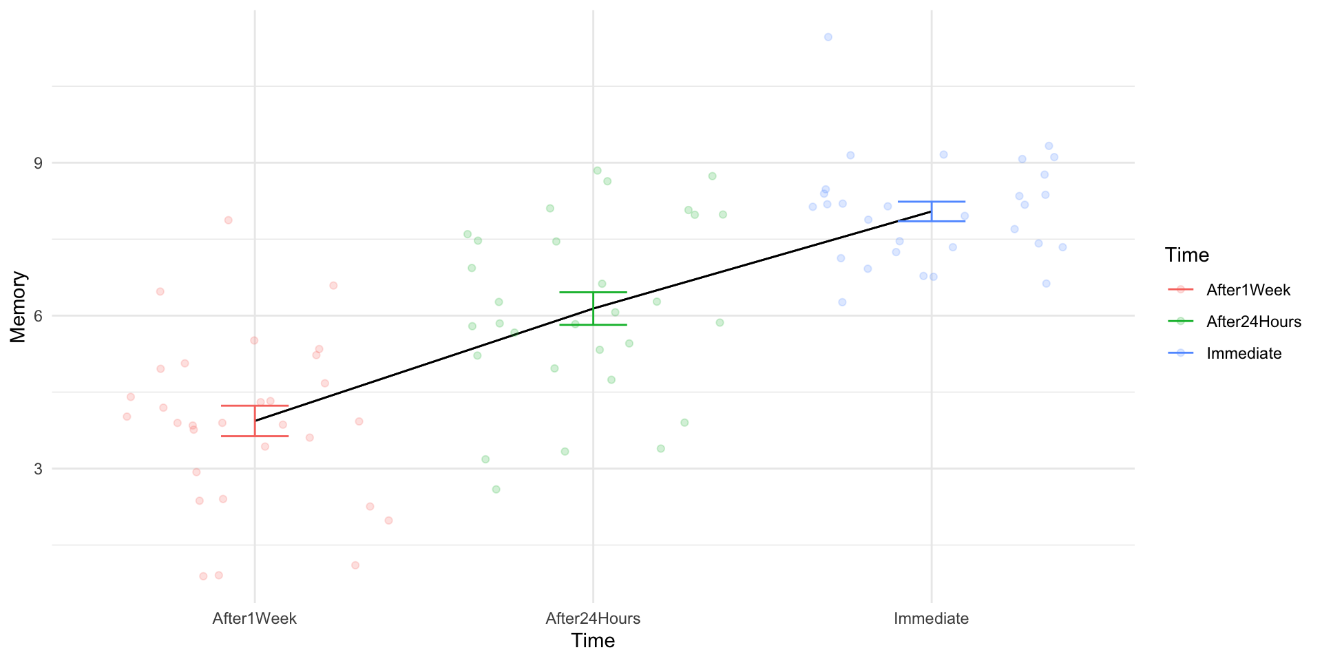
1. Memory Recall Study
Code
set.seed(100)# Memory Recall Studymemory_data <-data.frame(Participant =factor(1:30),Immediate =rnorm(30, mean =8, sd =1.5),After24Hours =rnorm(30, mean =6, sd =1.5),After1Week =rnorm(30, mean =4, sd =1.5))# Make Data Longermemory_data_long <- memory_data |> tidyr::pivot_longer(cols =!Participant,names_to ="Time",values_to ="Memory")aov(Memory ~ Time +Error(Participant), data = memory_data_long) |>tidy() |>mutate(Source = term,SS = sumsq,MS = meansq,`F`=ifelse(is.na(statistic),"--",statistic |>round(3)),p =ifelse(p.value >.05,"<.05",p.value),p =ifelse(is.na(p),"--",p) ) |>select(Source, df, SS, MS, `F`, p) |>gt() |>fmt_auto()