Linear Regression
PSY 348: Lecture 16
Dave Brocker
Farmingdale State College
Types of Analysis
looks_one
Univariate
One variable, like the mean
looks_two
Bivariate
Two variables, like correlation
looks_3
Multivariate
More than 2 variables
Regression
How regression relates to correlation
Regression is the multivariate version of correlation.
Correlation is the bivariate version of regression.
We’re doing the same thing in regression as we do in correlation, BUT we can have more than 2 variables.
Regression terminology
Outcome and predictors
- \(Y\)
- The outcome variable: the one we choose to predict.
- \(\hat{Y}\)
- The predicted value of \(Y\) from the model.
- \(A\), \(B\), etc.
- The predictor variables we have reason to believe predict \(Y\) (one or more).
Regression terminology
- Regress
- When we predict \(Y\) with \(X\), we say that we regress \(Y\) on \(X\).
Regression Equation
Step-by-step
\[ \large{\color{red}{Y_i} = \color{green}{\beta_0} + \color{blue}{\beta_1(A)}+\color{orange}{e_i}} \]
1. The observed value of \(Y\) for a particular participant (\(i\))
2. Intercept: the predicted \(Y\) when all predictors are 0
3. Coefficient (weight): the predicted change in \(Y\) for a one-unit increase in \(A\)
4. The value of a particular participant on the measure of \(A\)
5. Error: random, and therefore cannot be predicted
Regression Equation
A few ways to write the same thing
\[ \large{\color{red}{Y_i} = \color{green}{\beta_0} + \color{blue}{\beta_1(A)} + e_i} \]
\[\hat{Y} = \beta_0 + \beta_1(A)\]
\[Y = a + bX\]
Linear Regression
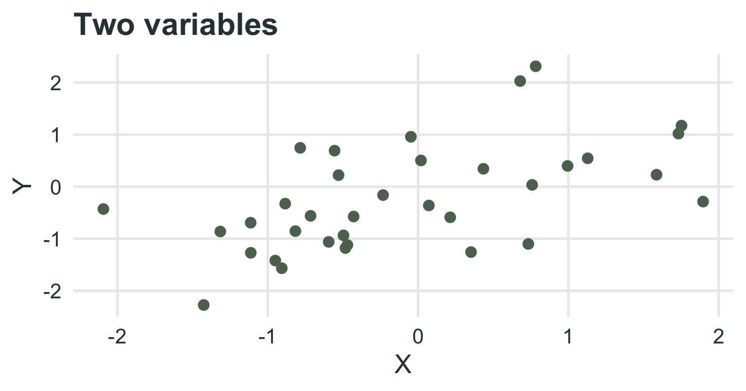
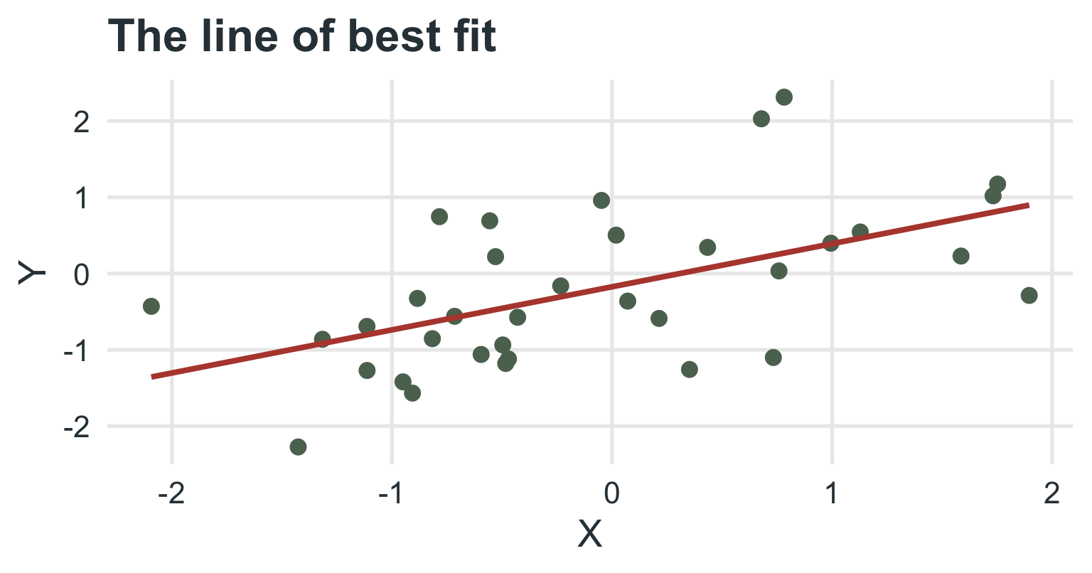
Line of best fit
Linear Regression
Least squares
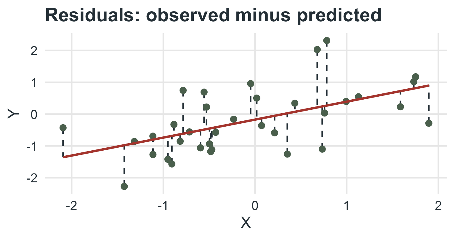
The line of best fit is the line that makes the residuals as small as possible.
A residual is the distance between an observed \(Y\) and its predicted \(\hat{Y}\): \(e_i = Y_i - \hat{Y}_i\).
Least squares picks the line that minimizes the sum of the squared residuals, \(\sum e_i^2\).
Regression
Equation component meanings
\(Y\) = the actual, observed \(y\) value for a participant
\(\hat{Y}\) = the model’s predicted \(y\) value for a participant
\(\beta_0\) = the intercept: the predicted \(y\) when \(A\) is 0
\(A\) = the \(A\) value for a participant
\(\beta_1\) = the coefficient for \(A\): it is multiplied by \(A\) and added to \(\beta_0\) to estimate \(y\)
Regression Equation
More than one X
Multiple regression
\(\large{\hat{Y}_i = \beta_0 + \beta_1(A) + \beta_2(B) + \cdots}\)
\(\beta_1\) and \(\beta_2\) are the coefficients for predictors \(A\) and \(B\).
Each coefficient is the predicted change in \(Y\) for a one-unit increase in that predictor, holding the other predictors constant.
Regression in R
The lm() function
regression.R
Call:
lm(formula = Social_Media_Use ~ Age + Sense_of_Belonging, data = df_sob)

Residuals:
     Min       1Q   Median       3Q      Max
-0.75174 -0.42669 -0.06621  0.33997  0.96242

Coefficients:
                   Estimate Std. Error t value Pr(>|t|)
(Intercept)         5.22914    0.42914  12.185 1.75e-12 ***
Age                -0.10346    0.01058  -9.775 2.31e-10 ***
Sense_of_Belonging  0.29033    0.03570   8.133 9.78e-09 ***
---
Signif. codes:  0 '***' 0.001 '**' 0.01 '*' 0.05 '.' 0.1 ' ' 1

Residual standard error: 0.512 on 27 degrees of freedom
Multiple R-squared:  0.8704,    Adjusted R-squared:  0.8608
F-statistic: 90.68 on 2 and 27 DF,  p-value: 1.046e-12
Interpreting Coefficients
Regression Model Table
Two predictor variables
| Characteristic | Beta | 95% CI | p-value |
|---|---|---|---|
| (Intercept) | 5.2 | 4.3, 6.1 | <0.001 |
| Age | -0.10 | -0.13, -0.08 | <0.001 |
| Sense_of_Belonging | 0.29 | 0.22, 0.36 | <0.001 |
| Abbreviation: CI = Confidence Interval | |||
Interpreting coefficients
- Beta (\(b\))
- The predicted change in \(y\) for a one-unit increase in the predictor, holding the other predictors constant.
- t-value
- The coefficient divided by its standard error: \(t = b / SE_b\).
- p-value
- Is this a significant predictor of \(y\)?
To compare which predictor matters more, use standardized betas. Unstandardized betas depend on the units of each predictor (years vs. a 0 to 10 scale).
\(R^2\): Coefficient of Determination
How much can we account for?
\(R^2\) is the correlation coefficient (\(r\)) squared, and is always between 0 and 1.
In correlation, it is the amount of \(y\) accounted for by \(x\).
In regression, \(R^2\) is the amount of \(y\) accounted for by all of the predictors together.
Did we account for a significant amount of the variance in \(y\)?
Interpreting R Squared
- \(R^2\)
- The percentage of \(y\) accounted for by the predictors.
- Adjusted \(R^2\)
- The same, but penalized for using too many predictors.
- F-value and p-value
- Is the model as a whole a significant predictor of \(y\)?
The Formulas Behind These
\[R^2 = 1 - \dfrac{SS_{residual}}{SS_{total}} = \dfrac{SS_{model}}{SS_{total}}\]
\[R^2_{adj} = 1 - (1 - R^2)\dfrac{n-1}{n-p-1} \qquad F = \dfrac{R^2 / p}{(1 - R^2)/(n - p - 1)}\]
- \(SS_{residual}\) is the variation in \(y\) the model leaves unexplained; \(SS_{total}\) is all the variation in \(y\)
- \(n\) is the sample size and \(p\) is the number of predictors
- \(F\) is variance explained per predictor, divided by variance left unexplained per remaining df
Assumptions of Linear Regression
Assumptions
- Linearity: the relationship between each predictor and \(y\) is linear.
- Independence: the observations (and residuals) are independent.
- Homoscedasticity: the residuals have about the same spread at every predicted value.
- Normality: the residuals are approximately normal.
- No severe multicollinearity: the predictors are not nearly duplicates of one another.
Linear Regression Example
Linear Regression
Example
Professor Brocker wants to be able to predict social media use. The Social Media Use Scale measures different motivations and reasons for using Social Media platforms.
What are some predictors of social media use?
Sense of belonging
Age
Regression Equation
Theoretical
\[\large{\color{red}{Y_i} = \color{green}{\beta_0} + \color{orange}{\beta_1}\color{blue}{(Age)} + \color{purple}{\beta_2(SOB)} + e_i}\]
The observed degree of social media use for a participant “\(i\)”
Intercept: predicted social media use when all other predictors are 0
Coefficient for Age (\(\beta_1\))
The participant’s age
Coefficient for Sense of Belonging (\(\beta_2\))
The participant’s sense of belonging
Randomness
Example
Model coefficients
| Social Media Use Model | |||
| Characteristic | Beta | 95% CI | p-value |
|---|---|---|---|
| (Intercept) | 5.2 | 4.3, 6.1 | <0.001 |
| Age | -0.10 | -0.13, -0.08 | <0.001 |
| Sense_of_Belonging | 0.29 | 0.22, 0.36 | <0.001 |
| Abbreviation: CI = Confidence Interval | |||
Example
Model summary
| Regression Model Summary | |
| Predicting social media use from age and sense of belonging | |
| Metric | Value |
|---|---|
| Residual Standard Error | 0.512 |
| Multiple R-squared | 0.870 |
| Adjusted R-squared | 0.861 |
| F-statistic | 90.681 |
| p | 0.000 |
Reporting Regression Findings
Reporting
The overall model
First, report adjusted \(R^2\) and its corresponding \(p\):
Age and sense of belonging predicted a significant amount of variance in social media use, adjusted \(R^2\) = 0.86, F(2, 27) = 90.68, p < .001.
Reporting
The individual predictors
Then report individual betas and their \(p\)’s:
Sense of belonging significantly predicted social media use (b = 0.29, p < .001), and so did age (b = -0.10, p < .001).
It’s common to report betas and \(p\)’s in the text and in a table.
Interpretation: for each additional year of age, predicted social media use drops by 0.10 hours per day, holding sense of belonging constant.
Categorical Variables in Regression
Multiple Predictors
Understanding the factors that influence energy levels
What determines how energized you feel throughout the day? Is it the number of cups of coffee you drink? The amount of sleep you got the night before? Or maybe even the type of TV shows you watch before bed?
Multiple Predictors
Four predictors
We explore how TV watching habits (duration and genre), caffeine intake, and prior sleep predict energy levels:
Duration of TV watching (continuous): does more TV drain your energy?
Cups of coffee (continuous): does caffeine actually help?
Prior sleep (continuous): does more sleep mean more energy?
TV genre (categorical: Comedy, Drama, Documentary): can what you watch change how you feel?
Categorical Variables
Dummy coding
How R handles a categorical predictor
A variable with \(k\) categories becomes \(k - 1\) dummy variables (0/1). One category is the reference group, and each coefficient compares a category to the reference.
| TV genre | Drama | Documentary |
|---|---|---|
| Comedy (reference) | 0 | 0 |
| Drama | 1 | 0 |
| Documentary | 0 | 1 |
Fit the Model
| Energy Level Model | |||
| What is the best predictor? | |||
| Characteristic | Beta | 95% CI | p-value |
|---|---|---|---|
| (Intercept) | 1.7 | 0.32, 3.1 | 0.017 |
| Duration_TV | -0.63 | -0.87, -0.38 | <0.001 |
| Cups_of_Coffee | 0.62 | 0.43, 0.81 | <0.001 |
| Prior_Sleep | 0.73 | 0.56, 0.89 | <0.001 |
| TV_Genre | |||
| Comedy | — | — | |
| Drama | -0.97 | -1.9, -0.06 | 0.038 |
| Documentary | -1.3 | -1.9, -0.69 | <0.001 |
| Abbreviation: CI = Confidence Interval | |||
Interpreting a Categorical Predictor
Reading the genre coefficients
Drama: drama watchers have energy 0.97 points lower than comedy watchers (the reference), holding the other predictors constant.
Documentary: documentary watchers are 1.32 points lower than comedy watchers.
- The reference group does not get its own coefficient. Its mean is folded into the intercept.
Horror Movies
A real dataset
Does a film’s “scare score” predict its Rotten Tomatoes score, once we account for the year it was made and whether it is a sequel?
| Characteristic | Beta | 95% CI | p-value |
|---|---|---|---|
| Scare score | 0.18 | -0.20, 0.55 | 0.4 |
| Year | -0.15 | -0.60, 0.29 | 0.5 |
| Sequel (vs. not) | |||
| no | — | — | |
| yes | -12 | -27, 2.1 | 0.093 |
| Abbreviation: CI = Confidence Interval | |||
Horror Movies
Reading the model
The overall model is not significant: adjusted \(R^2\) = 0.05, F(3, 46) = 1.80, p = .160.
None of the predictors reaches significance (the sequel coefficient is closest, p = .093).
Not every plausible predictor works: how scary a film is does not predict how critics rate it.
Horror Movies
A warning about circular predictors
Be careful what goes in the model
If we predict the scare score from the heart-rate measures in the same dataset, we get a nearly perfect model: \(R^2\) = 0.997.
That looks circular, not like a discovery: the scare score appears to be computed from those measures. Predictors that are derived from the outcome (like a movie’s ranking) or are exact combinations of one another (like overall difference = average movie heart rate minus resting heart rate) also cause problems, such as multicollinearity.
Review Questions
Multiple Choice
1. What does the slope in a simple linear regression equation represent?
The value of Y when X = 0
The predicted change in Y for a one-unit increase in X
The strength of the correlation between X and Y
The proportion of variance in Y explained by X
Answer: B
The slope is the predicted change in Y for a one-unit increase in X. (A is the intercept, C is \(r\), and D is \(R^2\).)
Multiple Choice
2. If a linear regression model has an R² value of 0.85, what does this mean?
85% of the variability in X is explained by Y
The regression model is 85% accurate
85% of the variability in Y is explained by X
The relationship between X and Y is statistically significant
Answer: C
\(R^2\) is the proportion of the variability in the outcome (Y) accounted for by the predictor(s). It says nothing by itself about statistical significance.
Multiple Choice
3. A researcher runs a regression and finds the equation \(\hat{Y} = 5 + 2X\). What does the number 5 represent?
The slope of the regression line
The predicted value of Y when X = 0
The effect size of X on Y
The p-value of the regression
Answer: B
5 is the intercept: the predicted Y when X = 0. (The slope is 2.)
Multiple Choice
4. Which of the following would indicate that a multiple regression model is overfitting?
A high R² value on the training data but poor performance on new data
A non-significant p-value for the intercept
The presence of a negative coefficient in the model
A low standard error for the slope
Answer: A
An overfit model captures noise in the sample, so it looks great on the data it was fit to and predicts new data poorly.
Multiple Choice
5. A model predicts salary from years of experience. The p-value for the slope is 0.0003. What does this mean?
Years of experience does not significantly predict salary
Years of experience significantly predicts salary at the α = 0.05 level
The slope coefficient is 0.0003
The model is not linear
Answer: B
\(p < .05\), so years of experience is a significant predictor of salary.
Open-Ended Questions (Show Your Work)
Open-Ended
6. A multiple regression model
\(\hat{Y} = 3 + 1.5X_1 - 0.7X_2\)
\(X_1\) = number of hours spent studying
\(X_2\) = number of hours spent watching TV
a) Predict the outcome if a student studies for 6 hours and watches TV for 2 hours.
b) Interpret the coefficient of \(X_2\).
Answer
a) \(\hat{Y} = 3 + 1.5(6) - 0.7(2) = 3 + 9 - 1.4 = 10.6\)
b) For each additional hour of TV, the predicted outcome decreases by 0.7, holding hours of studying constant.
Open-Ended
7. A simple linear regression output
| Predictor | Coefficient | Std. Error | p-value |
|---|---|---|---|
| Intercept | 4.2 | .5 | .001 |
| X | 1.8 | .3 | .0005 |
a) Write the equation. b) Interpret the slope. c) Predict Y if X = 10.
Answer
a) \(\hat{Y} = 4.2 + 1.8X\)
b) For each one-unit increase in X, the predicted Y increases by 1.8, and the slope is significant (\(p = .0005\)).
c) \(\hat{Y} = 4.2 + 1.8(10) = 22.2\)
Open-Ended
8. Sleep (X) and energy (Y): \(\hat{Y} = 2 + 3X\)
a) Interpret the slope.
b) Predict energy for a person who sleeps 7 hours.
c) Interpret the intercept. Is it meaningful here?
Answer
a) Each additional hour of sleep predicts 3 more points of energy.
b) \(\hat{Y} = 2 + 3(7) = 23\)
c) The intercept is the predicted energy for 0 hours of sleep. It is probably not meaningful, because nobody in the data sleeps 0 hours (that would be extrapolating).
Summary: Linear Regression
Regression predicts an outcome (\(Y\)) from one or more predictors: \(\hat{Y} = \beta_0 + \beta_1 A + \beta_2 B + \cdots\)
The line of best fit minimizes the squared residuals.
Each coefficient is the predicted change in \(Y\) for a one-unit increase in that predictor, holding the others constant.
\(R^2\) and adjusted \(R^2\) tell us how much of \(y\) the model accounts for, and the F-test tells us whether the model as a whole is significant.
Categorical predictors become dummy variables compared to a reference group.
Check the assumptions, and watch out for circular or collinear predictors.
Linear Regression | ⬡⬢⬡⬢⬡⬢