With a t-test, we were able to compare two means from independent samples, why not just do the same but for three independent samples?
Conceptually, imagine we have an Independent Variable with 3 levels (A,B,C). If we wanted to see if there was a difference we need to examine multiple comparisons.
\(A > B \| A > C\| B > C\)
ANOVA
Sampling Theory
Code
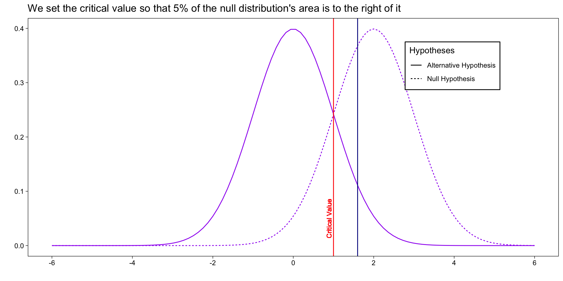
library(ggplot2)library(dplyr,warn.conflicts =FALSE)library(huxtable)library(tidyr)# Generate data for two normal distributionsx <-seq(-6, 6, length=100)null_dist <-dnorm(x, mean =0, sd =1)alt_dist <-dnorm(x, mean =2, sd =1)data <-data.frame(x =rep(x, 2),y =c(null_dist, alt_dist),hypothesis =factor(rep(c("Null Hypothesis", "Alternative Hypothesis"), each=length(x))))plt <-ggplot(data, aes(x = x, y = y, lty =rev(hypothesis))) +geom_line(aes(color ="purple")) +theme_linedraw() +labs(x ="",y ="",lty ="Hypotheses" ) +theme(panel.grid =element_blank(),legend.position ="inside",legend.position.inside =c(.8,.8),legend.background =element_rect(color ="black") ) +scale_color_identity()plt +geom_vline(xintercept =1.6,color ="darkblue" ) +geom_vline(xintercept =1, color ="red" ) +geom_text(x =1, y = .05, label ="Critical Value",color ="red",angle =90,size =3,vjust =-.4 ) +scale_x_continuous(breaks =c(-6,-4,-2,0,2,4,6) ) +labs(title ="We set the critical value so that 5% of the null distribution's area is to the right of it")
ANOVA
The Types
There are 3 types of ANOVA:
Between-Subjects
Within subjects (repeated measures ANOVA)
Mixed designs (between and within together)
ANOVA
The Types
There are 3 types of ANOVA:
One Factor (1 IV)
Factorial (2+ IV)
MANOVA
Between Subjects ANOVA
Between Subjects ANOVA
Definition
The Independent Samples t-test was an example of Between Subjects experimental design
Between-Subjects designs are also known as Independent Group Designs as they utilize the same principles
Participants are randomly assigned to each level of the Independent Variable making their scores independent from each other
Between Subjects ANOVA
Example
The experimental group drinks caffeinated coffee. The placebo group drinks decaf. The control group drinks water. I ask all 3 groups to complete a survey to measure their happiness on a scale of 1 to 10.
What is the IV?
How many levels does the IV have?
What is the DV?
Between Subjects ANOVA
Example
The experimental group drinks caffeinated coffee. The placebo group drinks decaf. The control group drinks water. I ask all 3 groups to complete a survey to measure their happiness on a scale of 1 to 10.
IV: Coffee Consumption
3 Levels: Coffee, Decaf, Water
DV: Happiness Score (1-10)
Between Subjects ANOVA
Example
The experimental group drinks caffeinated coffee. The placebo group drinks decaf. The control group drinks water. I ask all 3 groups to complete a survey to measure their happiness on a scale of 1 to 10.
The experimental group has a mean happiness score: 8
The placebo group mean happiness score: 6
The control group mean happiness score: 5
Between Subjects ANOVA
Example
Is the group that drank coffee significantly happier than the other groups?
If it’s all about the means, why is it called Analysis of Variance?
To compare the means, we analyzing two types of variance:
Variance among all of the scores (within group variance)
Variance between the groups (between group variance).
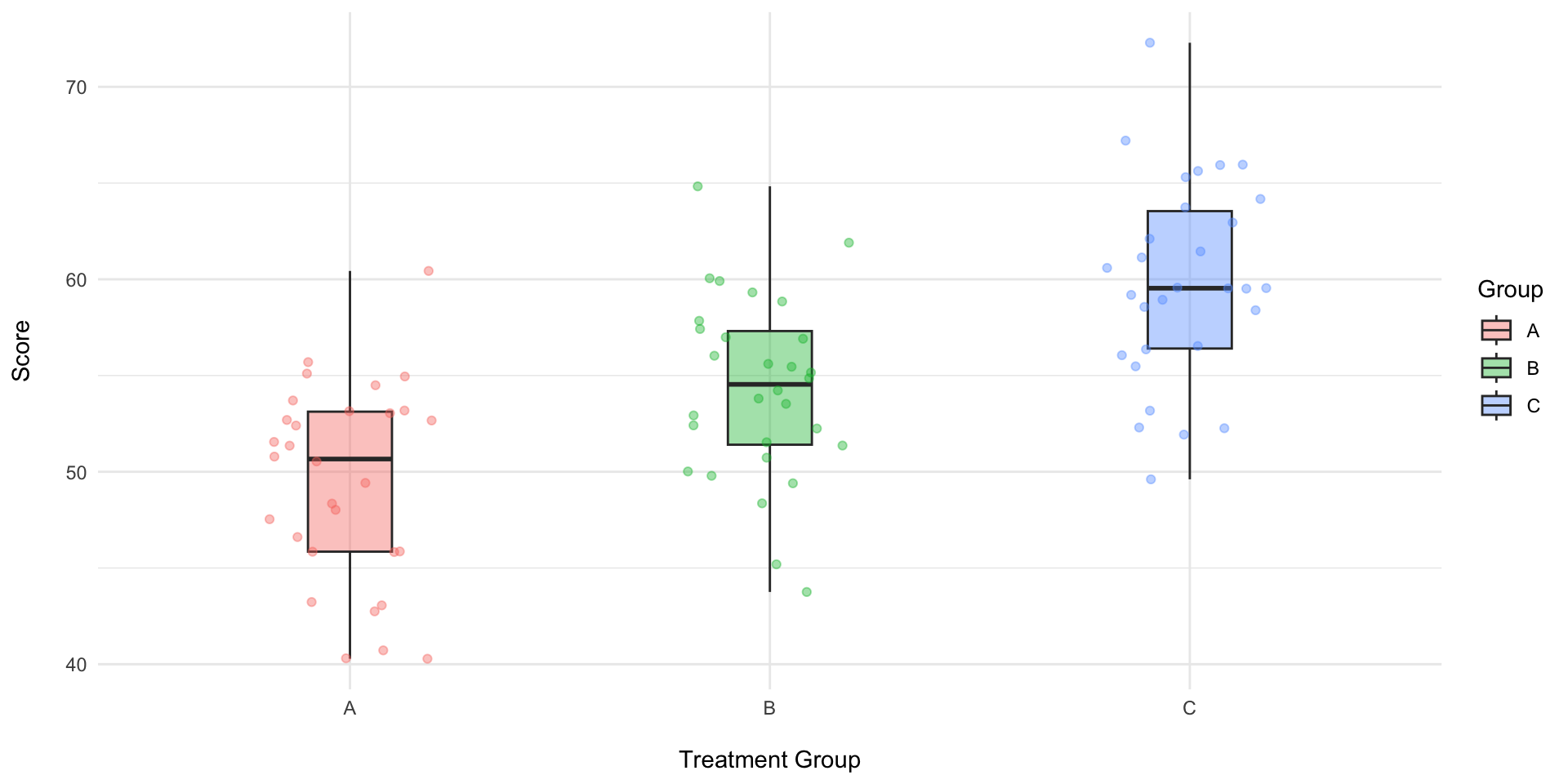
Between subjects ANOVA
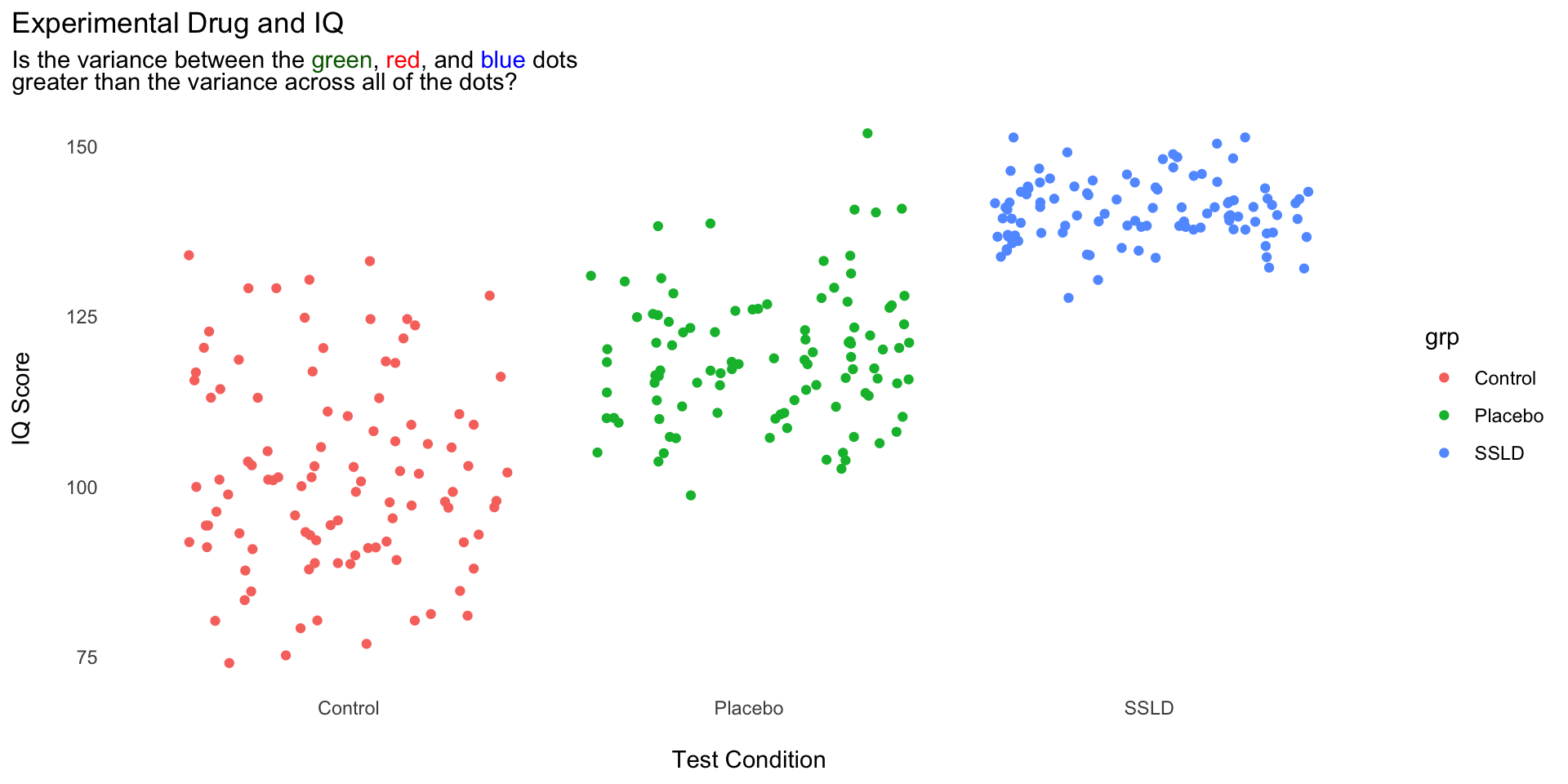
Visual
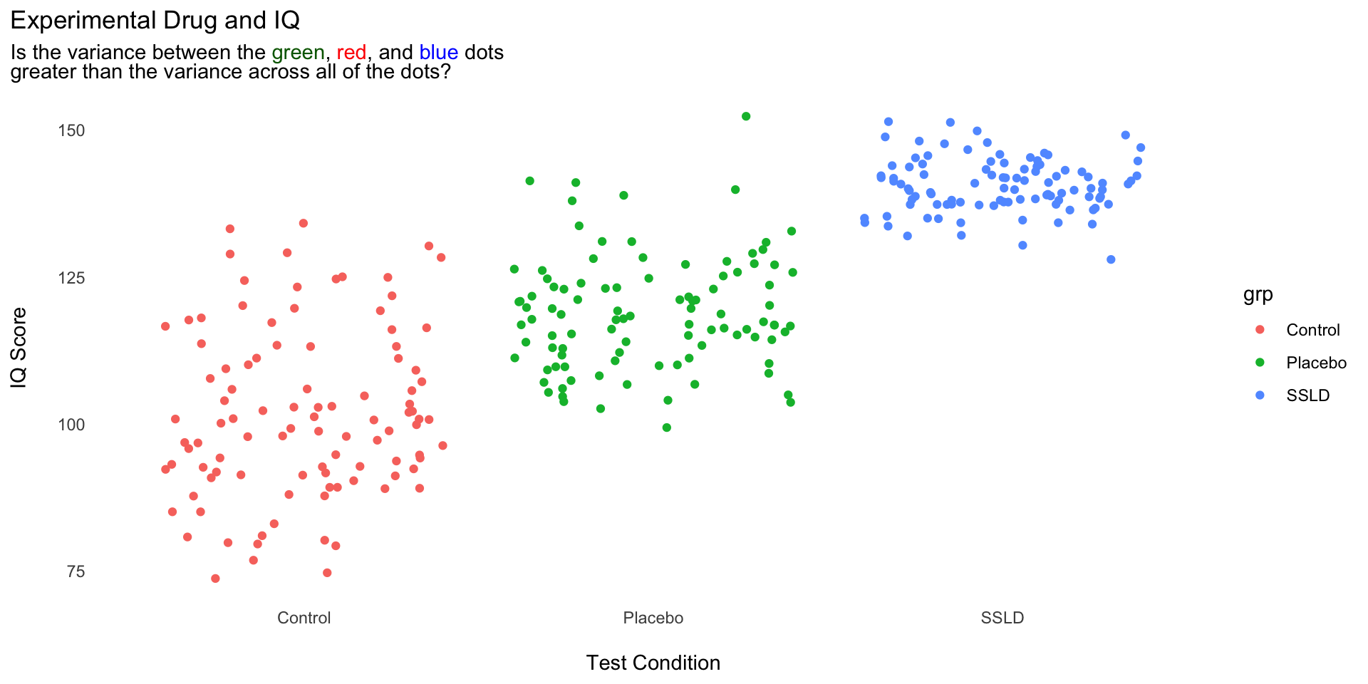
Code
set.seed(123)library(ggtext)exp <-tibble(grp =rep(c("SSLD","Placebo","Control"),each =100),IQ =c(rnorm(100,140,5),rnorm(100,120,10),rnorm(100,100,15)) |>round(0) )pl <- exp |>ggplot(aes(grp,IQ, color = grp)) +geom_jitter() +theme_minimal() +theme(panel.grid =element_blank(),plot.title.position ="plot",plot.subtitle =element_markdown() ) +labs(x ="\nTest Condition",y ="IQ Score\n",title ="Experimental Drug and IQ",subtitle ="Is the variance between the <span style = 'color:darkgreen'>green</span>, <span style = 'color:red'>red</span>, and <span style = 'color:blue'>blue </span>dots <br>greater than the variance across all of the dots?" )pl
library(broom)ano <-aov(IQ ~ grp, data = exp) |>tidy() |>rename(SS = sumsq,MS = meansq,`F`= statistic,p = p.value ) |>hux() |>set_align(value ="center") |>theme_article()ano[1,1] <-""ano[2:3,1] <-c("Between Groups","Within groups")anonew <- ano |>set_text_color(row =2, col =6, value ="red") |>set_number_format(fmt_pretty(digits =3)) anonew[2,6] <-"<.001**"anonew
df
SS
MS
F
p
Between Groups
2
75,293
37,647
355
<0.001**
Within groups
297
31,474
106
Calculating F
Calculating the variance
ANOVA looks at variance.
How do we calculate the Variance?
\(s^2 = \frac{\Sigma(x-\bar{x})^2}{n-1}\)
Calculating the variance
ANOVA looks at variance. To calculate the Variance:
Calculate the mean.
\(\frac{\sum x}{n}\)
Subtract the mean from each x-value - what is this called?
\((x-\bar{x})\)
Calculating the variance
ANOVA looks at variance. To calculate the Variance:
Calculate the mean.
Subtract the mean from each x-value (deviation score).
Square the deviation scores.
\((x-\bar{x})^2\)
Take the sum of the squared deviations - what is this called?
\(\Sigma (x-\bar{x})^2\)
Calculating the variance
ANOVA looks at variance. To calculate the Variance:
Calculate the mean.
Subtract the mean from each x-value (deviation score).
Square the deviation scores.
Take the sum of the squared deviations (Sum of Squared Deviations).
Calculating the variance
ANOVA looks at variance. To calculate the Variance:
Calculate the mean.
Subtract the mean from each x-value (deviation score).
Square the deviation scores.
Take the sum of the squared deviations (Sum of Squared Deviations).
Divide by (n-1) - what is this called?
Calculating the variance in ANOVA
To calculate the Variance in ANOVA:
Calculate the mean.
Subtract the mean from each x-value (deviation score).
Square the deviation scores.
Take the sum of the squared deviations (Sum of Squared Deviations).
Divide by (degrees of freedom).
This is the variance, but in ANOVA we also call it a Mean Squared (MS).
Calculating Means squared (MS)
Code
# Calculate the Sum of Squares (SS).ssex <-tibble(X =c(1,2,2,3,4,4,5,5,5,5,5,5,5,5,6,6,7,7,8,10),`x-xbar`= X -mean(X),`(X-xbar)^2`=`x-xbar`^2)# Show Datassex |>hux() |>theme_article() |>set_width(.8)
X
x-xbar
(X-xbar)^2
1
-4
16
2
-3
9
2
-3
9
3
-2
4
4
-1
1
4
-1
1
5
0
0
5
0
0
5
0
0
5
0
0
5
0
0
5
0
0
5
0
0
5
0
0
6
1
1
6
1
1
7
2
4
7
2
4
8
3
9
10
5
25
Code
# Divide the SS by the degrees of freedom.ss <-sum(ssex$`(X-xbar)^2`)# Show SSss
[1] 84
Code
ss/(length(ssex$X)-1)
[1] 4.421053
Calculating Means squared (MS)
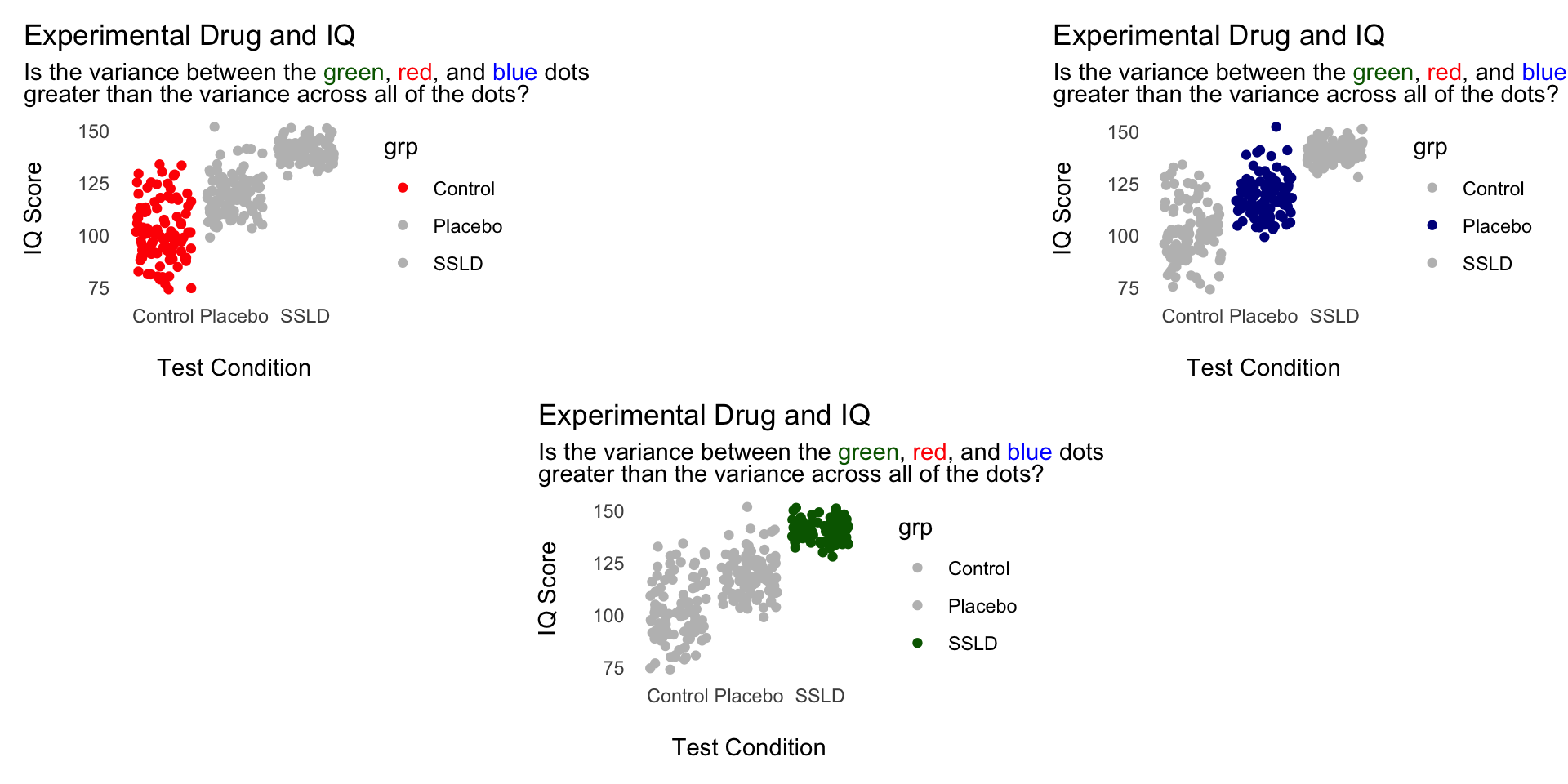
We will calculate a SS for the between group variance.
How much variance in the data is from group differences?
We will calculate a SS for all the data.
How much variance in the data is from random error?
Between subjects ANOVA
\(SS_{BG}\) = How much variance comes comes from the group differences?
\(SS_{Error}\) = How much variance is there in total among all the data points?
Code
pl
Calculating means squared (MS)
Calculate the \(SS_{BG}\)
Calculate the \(SS_{Error}\)
Divide the \(SS\) by their degrees of freedom.
Degrees of Freedom (df)
What Does it All Mean!
The number of observations (data points) in the data that are free to vary when estimating a statistic.
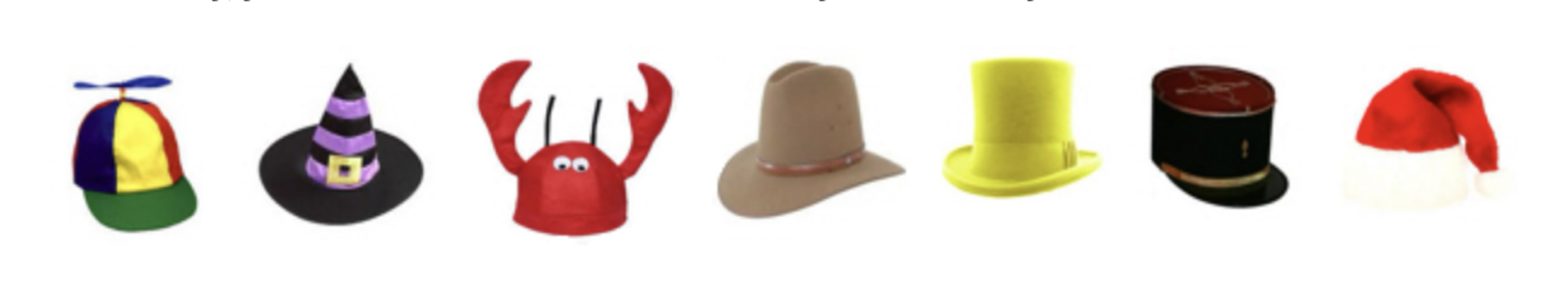
I own 7 hats. I want to wear a different hat every day of the week.
Degrees of Freedom (df)
What Does it All Mean!
On Monday, I have 7 hats to choose from.
On Tuesday, I have 6 hats to choose from.
On Wednesday, I have 5 hats to choose from.
On Thursday, I have 4 hats to choose from.
On Friday, I have 3 hats to choose from.
On Saturday, I have 2 hats to choose from.
Degrees of Freedom (df)
What Does it All Mean!
On Sunday, I don’t get a choice. On Sunday, I have to wear the Santa hat.
Degrees of Freedom (df)
What Does it All Mean!
The number of observations (data points) in the data that are free to vary when estimating a statistic.
The degrees of freedom is how many times I get a choice before I’m stuck with what’s left over.
Degrees of freedom
Between Groups (\(df_{BG} = k - 1\))
k is the number of groups in the independent variable.
Within Groups (\(df_{WG} = n - k\))
\(Total = n - 1\)
Calculating Means Squared (MS)
Calculate the \(SS_{BG}\).
Calculate the \(SS_{Error}\).
Divide the SS by their degrees of freedom.
Calculating the MS
Between Group Mean Squared: \(MS_{BG} = \frac{SS_{BG}}{k - 1}\)
Error Mean Squared: \(MS_{Error} = \frac{SS_{Error} }{(n - k)}\)
Prof Brocker gives one group of 100 participants the Super Secret Limitless Drug (SSLD). He gives another group of 100 participants a placebo. He gives the third group of 100 participants nothing. All participants then complete an IQ test. He wants to know if those who took the SSLD has significantly higher IQ than the placebo and the control groups.
Prof Brocker recruits 500 participants. He shows half of them the Netflix Original, Dark and the other half Jeopardy. He then measures their happiness on a scale of 1 to 10. He wants to know if Dark participants are significantly happier than the Jeopardy participants.
What is the IV?
What is the DV?
What is the sample size?
Interpreting F
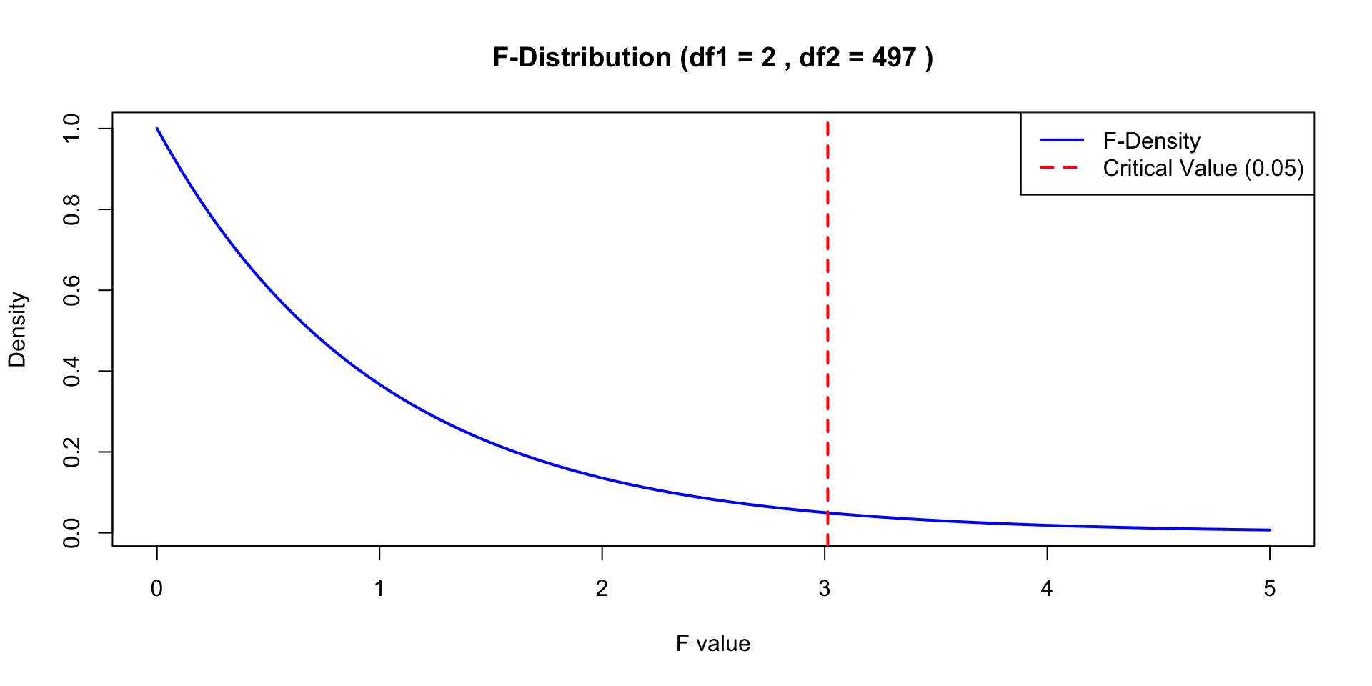
F-Distribution
Code
# Define the degrees of freedomdf1 <-2# Numerator degrees of freedomdf2 <-497# Denominator degrees of freedom# Plot the F-distribution curvecurve(df(x, df1, df2), from =0, to =5, col ="blue", lwd =2,xlab ="F value", ylab ="Density",main =paste("F-Distribution (df1 =", df1, ", df2 =", df2, ")"))# Add a vertical line at the critical value (e.g., 0.05 significance level)critical_value <-qf(0.95, df1, df2)abline(v = critical_value, col ="red", lwd =2, lty =2)# Add a legendlegend("topright", legend =c("F-Density", "Critical Value (0.05)"),col =c("blue", "red"), lwd =2, lty =c(1, 2))
Interpreting f
The \(MS_{BG}\) is made up of the \(MS_{Error}\) + the theoretical difference between groups:
\(F \gt 1\): Refer to p-value: Reject the Null Hypothesis
Reporting F
Reporting F
If asked to report findings in terms of the Null Hypothesis (\(H_0\)), you should report findings as:
Reject \(H_0\)
Fail to Reject \(H_0\)
Reporting F
What to Look For
If asked to report findings in general or for publication, you need to report 5 things:
\(F(df_{bg},df_{error})\)
F-value
p-value
Mean and standard deviation of each group
Reporting F
The group that watched Dark (M=8.43, s=1.02) reported significantly more happiness compared to their peers in the control group who watched Jeopardy (M=6.12, s=0.98), F(1,498) = 7.12, p < 0.05.
Reporting F
There was not a significant difference in happiness between the groups, \(F(1, 498) = 1.02, p = 0.07\).