PSY 348: Lecture 15
Farmingdale State College
What are measures of dispersion?
How spread out the data are: how much participants differ.
How did we measure dispersion when we were looking at one variable?
looks_one
Uni = one variable
looks_two
Bi = two variables
looks_3
Multi = more than two variables
Univariate
Standard deviation: how different are participants from the average?
Height: \(M = 5'6"\), \(s = 2\) inches
Bivariate
Covariance: do the variables vary in the same way?
Does the spread-out-ness of height overlap with the spread-out-ness of weight?
Professor Brocker wants to know if how many cups of coffee a professor drinks daily impacts their happiness. He asks
50professors how many cups they have in a typical day and then has them rate their happiness on a scale of1 to 10.
Variable 1: number of cups of coffee (continuous)
Variable 2: happiness (continuous)
The variance of each variable on its own.
The covariance of the two variables together.
Covariance
\(COV_{XY} = \dfrac{\Sigma(X-\bar{X})(Y-\bar{Y})}{N-1}\)
Well, well, well… we meet again
\(s^2 = \dfrac{\Sigma(X-\bar{X})^2}{N-1} = \dfrac{\Sigma(X-\bar{X})(X-\bar{X})}{N-1}\)
Steps
| Professor | X (cups) | Y (happiness) | X - mean(X) | Y - mean(Y) | Product | |
|---|---|---|---|---|---|---|
| 1 | 1 | 4 | −2.00 | −2.33 | 4.67 | |
| 2 | 2 | 5 | −1.00 | −1.33 | 1.33 | |
| 3 | 2 | 6 | −1.00 | −0.33 | 0.33 | |
| 4 | 3 | 6 | 0.00 | −0.33 | 0.00 | |
| 5 | 4 | 8 | 1.00 | 1.67 | 1.67 | |
| 6 | 6 | 9 | 3.00 | 2.67 | 8.00 | |
| Sum | — | — | — | — | — | 16.00 |
Covariance is the bivariate equivalent of variance.
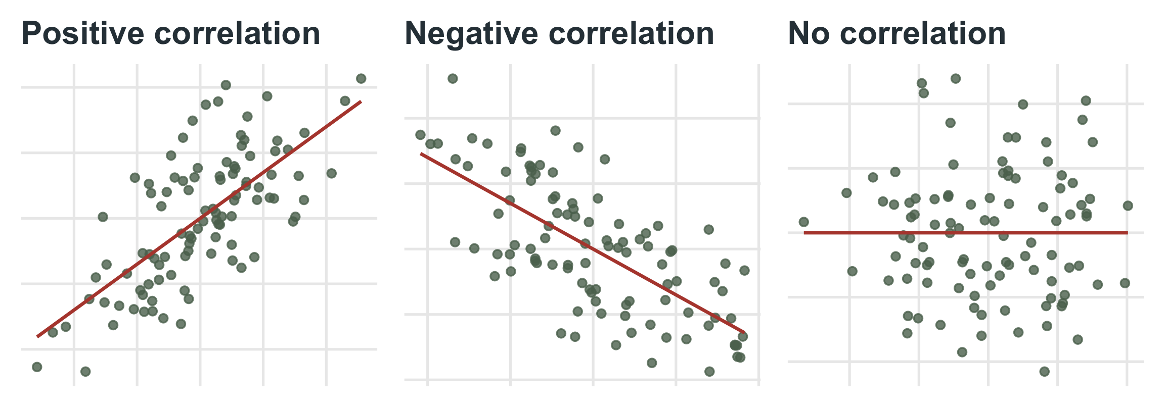
The sign tells us the direction: positive means the variables tend to rise together.
But the size is hard to interpret. It is in odd units (cups × happiness points) and changes if we change the scale.
Variance had the same problem (squared units), so we took the square root to get the standard deviation. For covariance, we standardize it.
Pearson correlation
\(r = \dfrac{cov_{xy}}{(SD_x)(SD_y)} = \dfrac{\Sigma(X-\bar{X})(Y-\bar{Y})}{(SD_x)(SD_y)(N-1)}\)
Correlation is the standardized covariance: we divide the covariance by the standard deviation of \(x\) times the standard deviation of \(y\).
Just as a z-score puts a score on a unit-free scale, \(r\) puts the relationship on a unit-free scale.
Compute r
\(r = \dfrac{cov_{xy}}{(SD_x)(SD_y)} = \dfrac{3.20}{(1.79)(1.86)} = 0.96\)
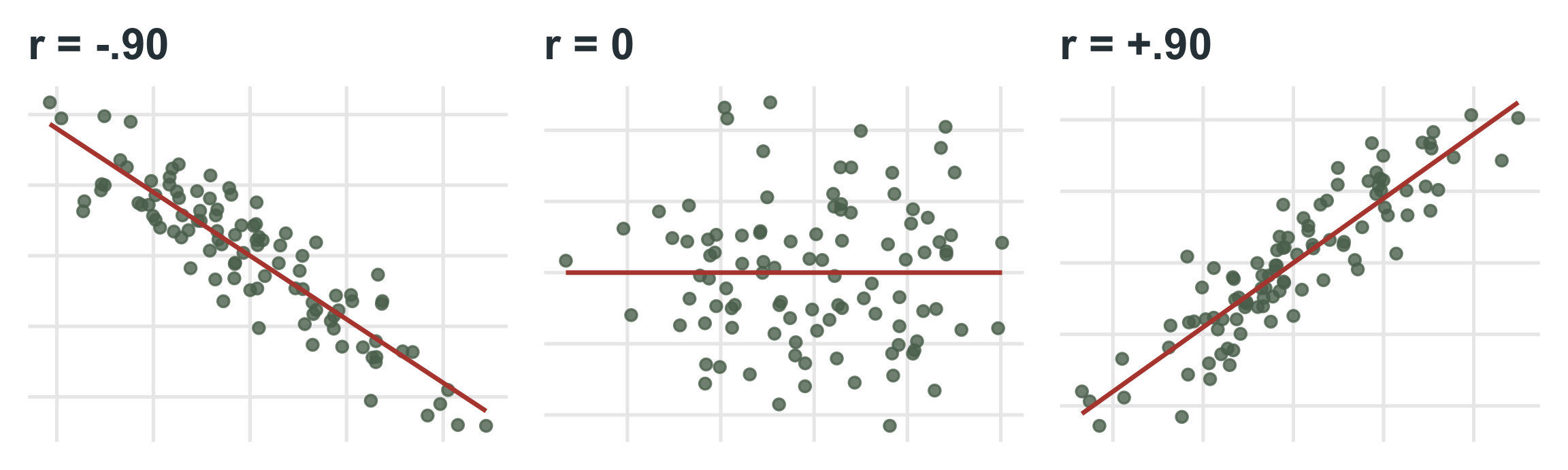
The sign indicates the direction.
The number indicates the magnitude (strength) of the relationship:
Rules of thumb
0.1 is a small correlation
0.3 is a moderate correlation
0.5 or higher is a large correlation
Correlation is written \(r\).
If we square \(r\), we get \(R^2\), which is always positive.
\(R^2\) is the proportion of variance the two variables share:
the amount of \(y\) accounted for by \(x\),
and the amount of \(x\) accounted for by \(y\).
Students’ grades in MTH 110 and their grades in this course correlate at \(r = 0.3\).
A moderate correlation.
How much of your grade in this course is accounted for by your MTH 110 grade?
Compute \(R^2\)
\(R^2 = r^2 = 0.3 \times 0.3 = 0.09\), so 9% of the variance in your grade is accounted for by your MTH 110 grade.
The test
\(t = \dfrac{r\sqrt{n-2}}{\sqrt{1-r^2}} \qquad df = n - 2\)
cor_test.R
Pearson's product-moment correlation
data: ex1$X and ex1$Y
t = 11.179, df = 48, p-value = 5.817e-15
alternative hypothesis: true correlation is not equal to 0
95 percent confidence interval:
0.7488197 0.9124630
sample estimates:
cor
0.85
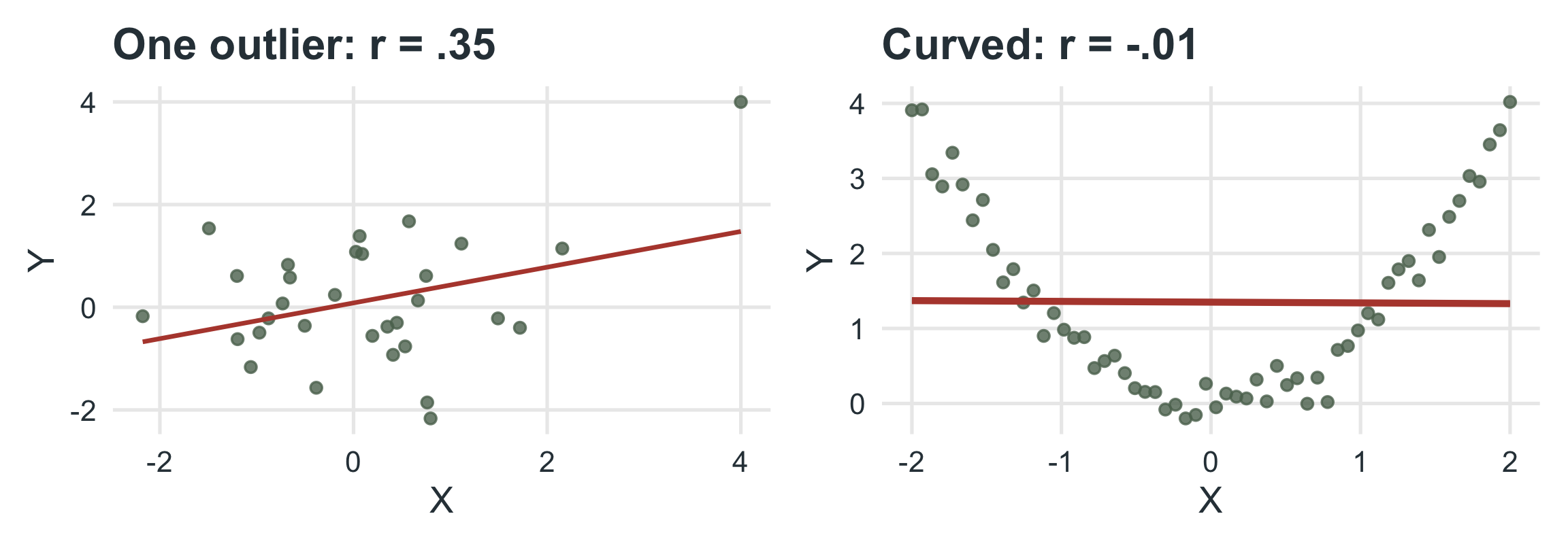
\(r\) measures linear relationships only, is pulled around by outliers, and shrinks when the range of one variable is restricted. Always plot your data.
In the Method, we report descriptive statistics about our variables (\(M\), \(s\)).
It is common to refer readers to a table where they can look at correlations between the variables.
Why might this be important?
Table 1 in a paper is typically a combination of descriptive stats and a correlation matrix:
| Variable | M | s | 1 | 2 | 3 |
|---|---|---|---|---|---|
| 1. Age | 20.91 | 1.76 | -- | -.03 | .65** |
| 2. Song 1 | 4.21 | 1.20 | -- | -.34* | |
| 3. Song 2 | 6.42 | 2.18 | -- | ||
| * p < .05. ** p < .01. | |||||
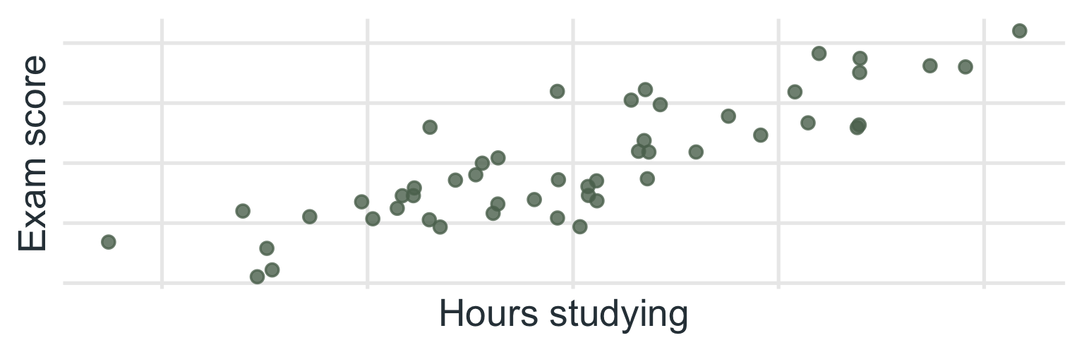
Researchers collected the hours spent studying and the final exam score for
50students (scatterplot below).
Answer
A strong, positive linear relationship: students who studied more hours tended to earn higher exam scores. In APA style: hours studying and exam scores were strongly positively correlated, r(48) = .85, p < .001.
Using the same data, the researchers fit a linear regression model to predict exam scores from the number of hours spent studying. The \(R^2\) value for the model is
0.72.
Your questions
Answers
Covariance is how two variables vary together: the bivariate equivalent of variance.
Correlation (\(r\)) is the standardized covariance: unit-free, bounded between -1 and +1.
The sign gives the direction and the size gives the strength; \(r^2\) is the shared variance.
Test \(H_0: \rho = 0\) with \(t = r\sqrt{n-2}/\sqrt{1-r^2}\), \(df = n - 2\).
Plot your data: outliers, curves and restricted ranges can fool \(r\).
Correlation does not imply causation.
Covariance & Correlation | ⬡⬢⬡⬢⬡⬢