PSY 348: Lecture 14
Farmingdale State College
Use Repeated Measures ANOVA when:
You have the same participants measured more than once (e.g., pre-test/post-test).
You’re interested in changes over time or under different conditions.
Between-subjects ANOVA
Compares means between groups (Group A vs. B vs. C).
Error comes from individual differences between people.
Within-subjects (repeated measures) ANOVA
Compares means within the same participants over time or conditions.
Controls for individual differences.
Can’t use multiple paired-samples t-tests.
Repeated-Measures ANOVA allows us to:
Compare within-subject changes across time.
Control for individual variability.
Test for an overall time effect.
Between-subjects ANOVA splits variance into between-group and error (within-group) parts.
Within-subjects ANOVA has a third source, because each person contributes several scores:
Removing the person
\(SS_{W} = SS_{Subjects} + SS_{Error}\)
\(SS_{Error} = SS_{W} - SS_{Subjects}\)
In between-subjects ANOVA, differences between people sit inside the error term.
In within-subjects ANOVA we subtract them out, so the error is smaller and the test is more powerful.
The F ratio
\(F = \dfrac{MS_{Time}}{MS_{Error}}\)
\(MS_{Time} = \dfrac{SS_{Time}}{df_{Time}} = \dfrac{SS_{Time}}{k - 1}\)
\(MS_{Error} = \dfrac{SS_{W} - SS_{Subjects}}{df_{Error}} = \dfrac{SS_{W} - SS_{Subjects}}{(n-1)(k-1)}\)
\(k\) is the number of time points (or conditions) and \(n\) is the number of participants.
Each SS is a sum of squared distances from a mean (\(\bar{x}_t\) = a time mean, \(\bar{x}_p\) = a person’s mean, \(\bar{x}_G\) = the grand mean): \(SS_{Time} = \sum n(\bar{x}_t - \bar{x}_G)^2 \quad SS_{Subjects} = \sum k(\bar{x}_p - \bar{x}_G)^2 \quad SS_{W} = \sum (x - \bar{x}_t)^2\)
Rules
Time: \(df_{Time} = k - 1\)
Subjects: \(df_{Subjects} = n - 1\)
Error: \(df_{Error} = (n - 1) \times (k - 1)\)
20 students rate their stress at three time points during finals week: three days before the exam, the night before, and after the exam.
What are the df’s for a one-way repeated-measures ANOVA on Time?
\(df_{Time} = 3 - 1 = 2\)
\(df_{Subjects} = 20 - 1 = 19\)
\(df_{Error} = 19 \times 2 = 38\)
| Source | df | SS | MS | F | p |
|---|---|---|---|---|---|
| Time (condition) | 2 | 105.58 | 52.79 | 69.19 | <.001 |
| Subjects | 29 | 175.71 | 6.06 | – | – |
| Error | 58 | 44.25 | 0.76 | – | – |
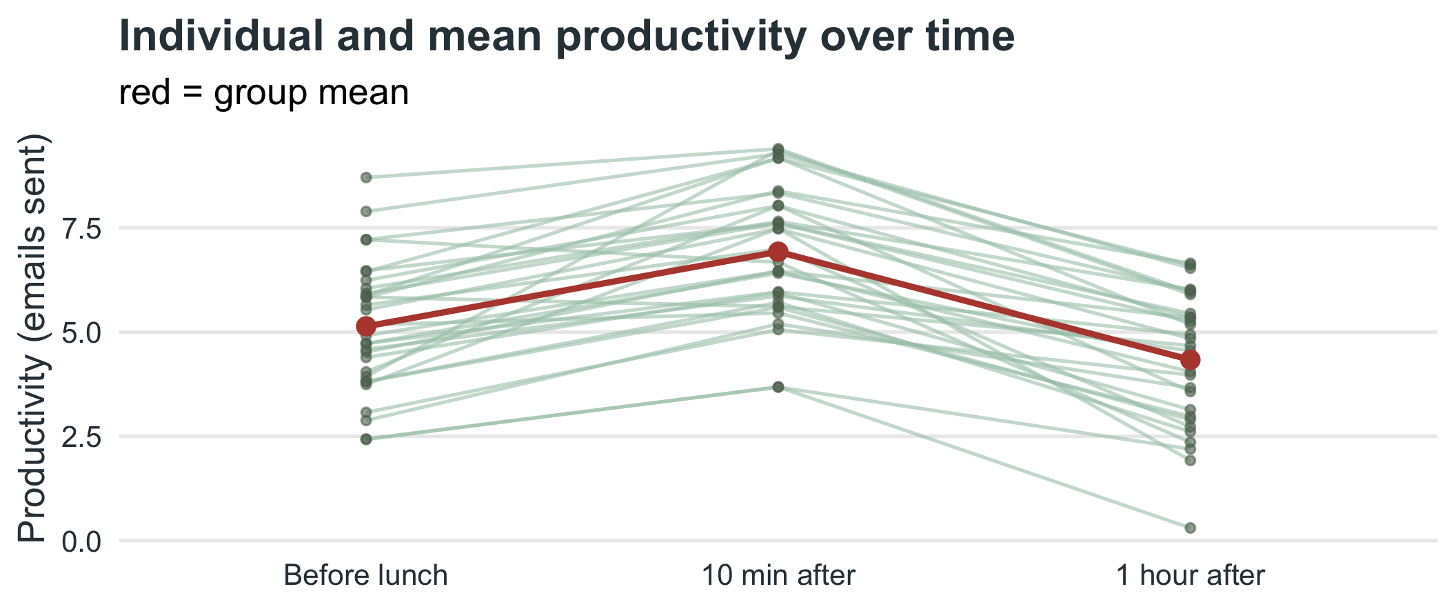
\(F(2, 58) = 69.19\), \(p\) < .001: productivity changes significantly across the three time points.
repeated_measures.R
Anova Table (Type 3 tests)
Response: y
num Df den Df MSE F ges Pr(>F)
cond 1.9264 55.866 0.79209 69.189 0.32431 1.403e-15 ***
---
Signif. codes: 0 '***' 0.001 '**' 0.01 '*' 0.05 '.' 0.1 ' ' 1
summary(fit) also prints Mauchly’s test and the other corrections.69.19
Repeated-measures F (removes person differences)
20.88
Between-subjects F (same data, ignoring the person)
Assumptions
Normality of the differences.
Sphericity: the variances of all pairwise differences are about equal.
If sphericity is violated, use the Greenhouse-Geisser correction.
\(F(2, 58) = 69.19\), \(p\) < .001
Main effect of time on productivity.
Productivity changes significantly across the timepoints.
Partial eta squared
\(\eta_p^2 = \dfrac{SS_{Time}}{SS_{Time} + SS_{Error}} = \dfrac{105.58}{105.58 + 44.25} =0.70\)
A significant F says that some time points differ, not which.
Run paired t-tests with a Bonferroni correction:
| Comparison | Adjusted p |
|---|---|
| Before lunch vs. 10 min after | <.001 |
| Before lunch vs. 1 hour after | 0.009 |
| 10 min after vs. 1 hour after | <.001 |
If asked to report findings in terms of the Null Hypothesis (H0), you should report findings as:
Reject \(H_0\), or
Fail to Reject \(H_0\)
If asked to report findings in general or for publication, you need to report \(F(df_{Time}, df_{Error}) = F, p\), an effect size, and the means and standard deviations at each time point.
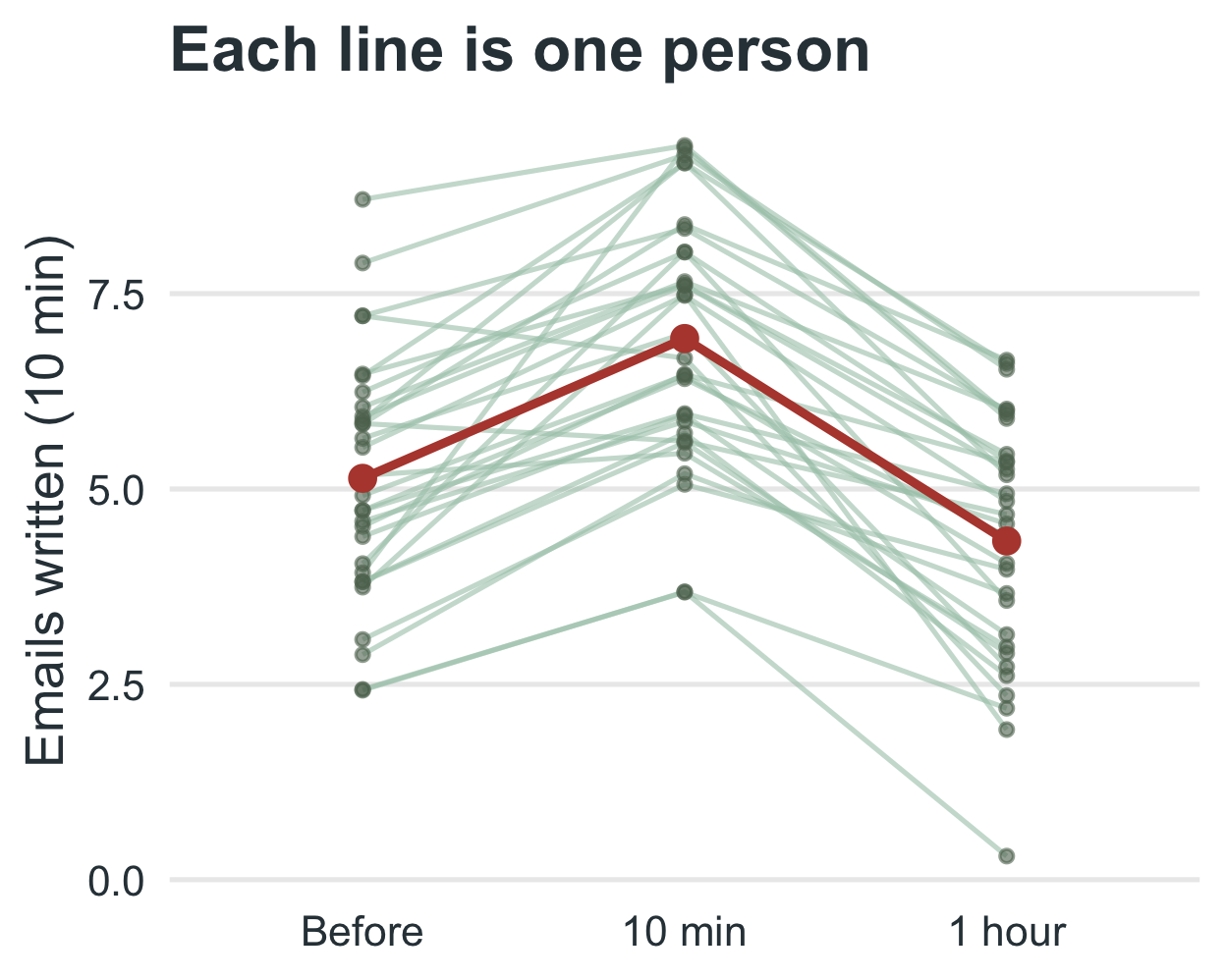
Productivity differed significantly across the three time points, F(2, 58) = 69.19, p < .001, \(\eta_p^2\) = 0.70. Productivity was highest 10 minutes after pizza (M = 6.93, SD = 1.61) and lowest an hour after pizza (M = 4.33, SD = 1.60); before lunch it was M = 5.14 (SD = 1.56).
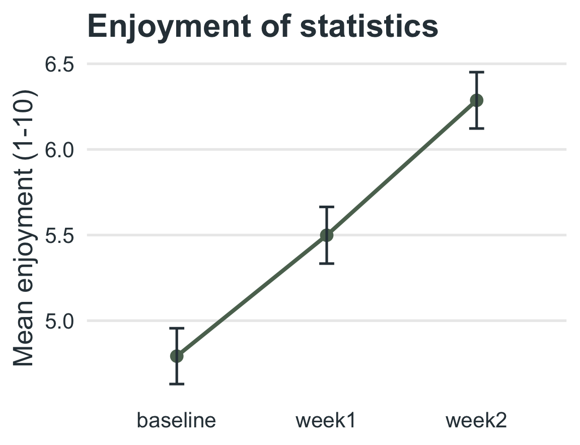
Prof. Brocker evaluates a new engagement intervention. 100 students rate their enjoyment of statistics (
1to10) at the start of the semester, after week 1 of a statistics warm-up activity, and after week 2.
Find the degrees of freedom
\(df_{Time}\) = ?
\(df_{Subjects}\) = ?
\(df_{Error}\) = ?
\(n\) = ?
Degrees of freedom
\(df_{Time} = k - 1 = 3 - 1 = 2\)
\(df_{Subjects} = n - 1 = 100 - 1 = 99\)
\(df_{Error} = (n - 1)(k - 1) = 99 \times 2 = 198\)
\(n = 100\)
Professor Brocker tests whether structured active-learning practices improve
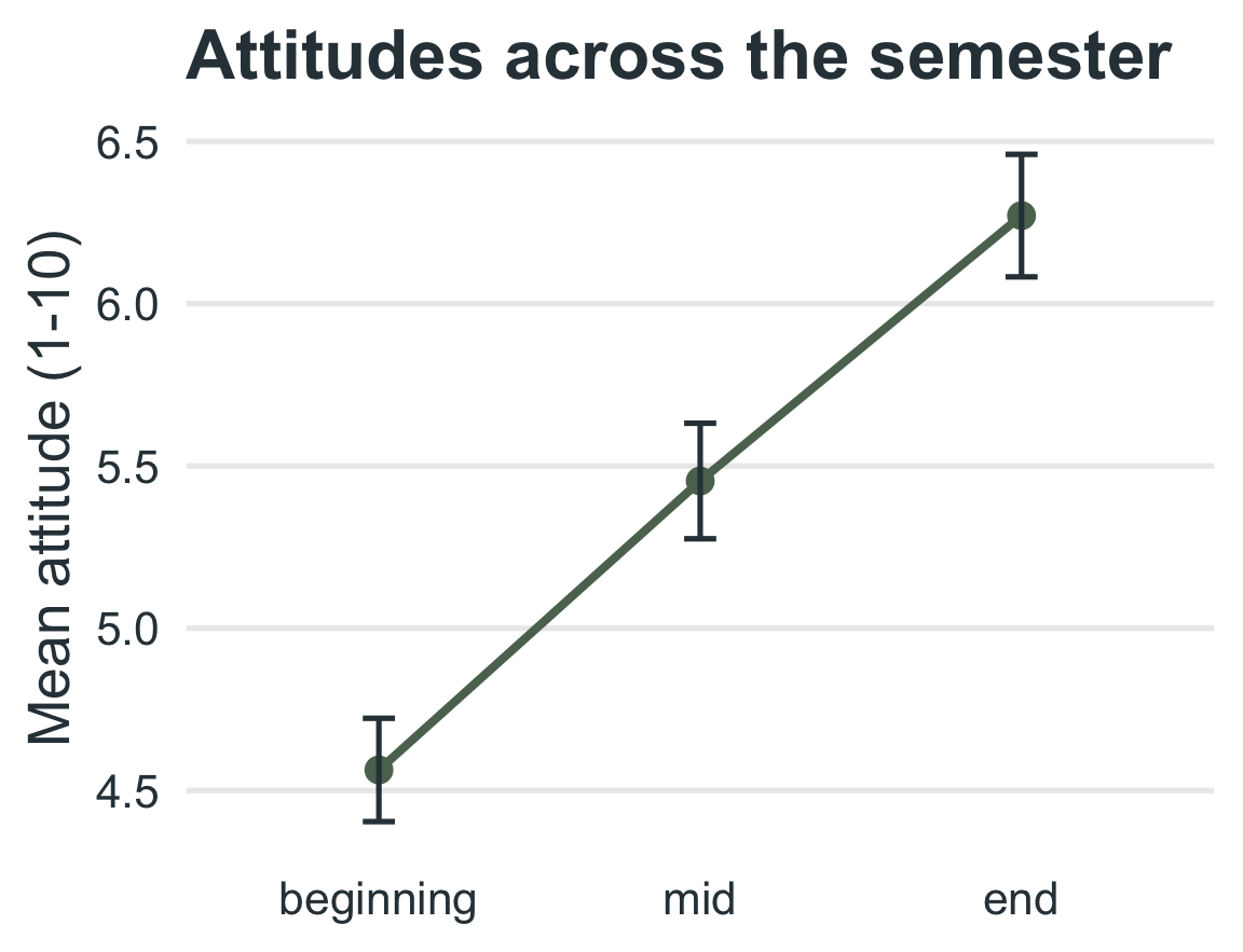
80students’ attitudes toward statistics. He collects a1-10enjoyment rating at the beginning of the semester, mid-semester (after four modules), and the end (after eight modules).
Find the degrees of freedom
Degrees of freedom
What F means
\(MS_{Time}\) is made up of \(MS_{Error}\) + the theoretical change over time:
\(MS_{Time} = \text{change over time} + MS_{Error}\)
If there is no change: \(MS_{Time} = 0 + MS_{Error}\), so \(F = \dfrac{MS_{Error}}{MS_{Error}} = 1\).
If there is a change: \(F = 1 + \dfrac{\text{change}}{MS_{Error}}\), which is greater than 1.
Decision rule
\(F \leq 1\): fail to reject the null hypothesis.
\(F > 1\): compare to the critical value (or use the p-value). Reject \(H_0\) only if \(p < \alpha\).
Attitudes toward statistics differed significantly across the semester, F(2, 158) = 281.96, p < .001. Attitudes were highest at the end of the semester (M = 6.27, SD = 1.69) and lowest at the beginning (M = 4.56, SD = 1.42). Mid-semester attitudes were M = 5.45 (SD = 1.59).
When collected, data can be in either wide or long format.
Below are the same five participants in both formats.
| Wide data | |||
| Each row is one participant | |||
| Participant | Immediate | After24Hours | After1Week |
|---|---|---|---|
| 1 | 11.4 | 4.6 | 4.5 |
| 2 | 6.2 | 7.1 | 8.1 |
| 3 | 7.0 | 5.8 | 7.4 |
| 4 | 7.4 | 6.2 | 4.5 |
| 5 | 6.5 | 9.3 | 6.8 |
| Long data | ||
| Each row is one participant at one time | ||
| Participant | Time | Memory |
|---|---|---|
| 1 | Immediate | 11.4 |
| 1 | After24Hours | 4.6 |
| 1 | After1Week | 4.5 |
| 2 | Immediate | 6.2 |
| 2 | After24Hours | 7.1 |
| 2 | After1Week | 8.1 |
| 3 | Immediate | 7.0 |
| 3 | After24Hours | 5.8 |
| 3 | After1Week | 7.4 |
| 4 | Immediate | 7.4 |
| 4 | After24Hours | 6.2 |
| 4 | After1Week | 4.5 |
| 5 | Immediate | 6.5 |
| 5 | After24Hours | 9.3 |
| 5 | After1Week | 6.8 |
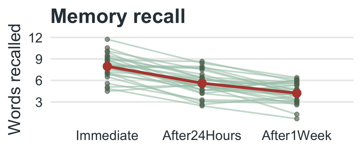
30 participants study a word list and recall it immediately, after 24 hours, and after 1 week. Does recall change over time?
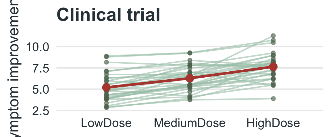
30 patients each receive a low, medium, and high dose of a medication (in separate sessions) and report symptom improvement. Does dose matter?
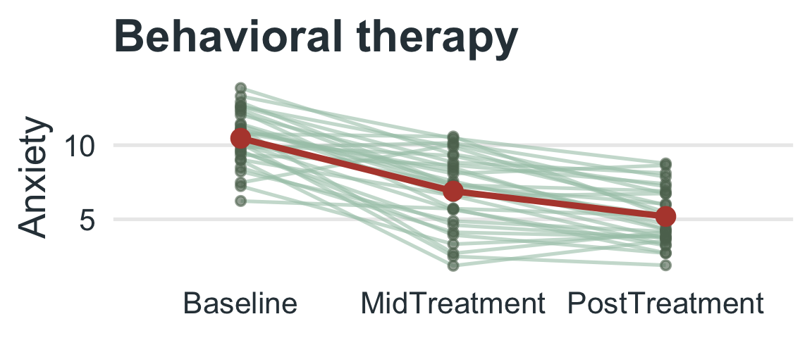
30 participants rate their anxiety at baseline, mid-treatment, and post-treatment.
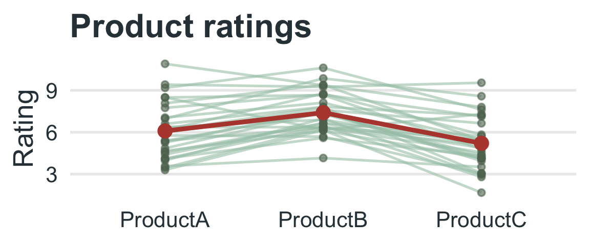
30 consumers each rate three products (A, B, and C).
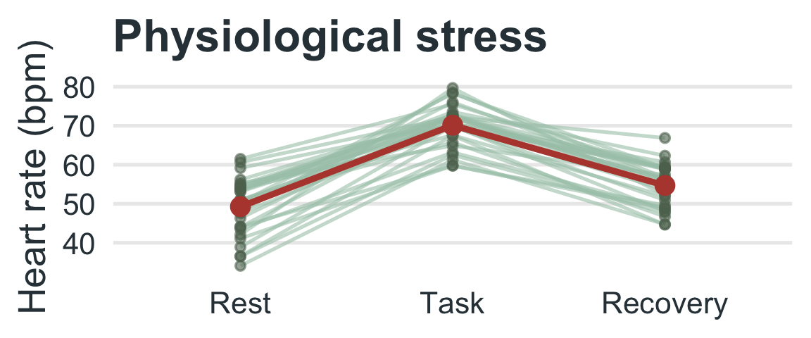
30 participants’ heart rate is measured at rest, during a task, and during recovery.
Compares three or more related means (the same people measured repeatedly).
Splits the variability into time, subjects, and error, and removes the subject differences from the error term.
\(F = MS_{Time} / MS_{Error}\) with \(df = (k - 1,\ (n - 1)(k - 1))\).
Check sphericity (Mauchly’s Test) and use the Greenhouse-Geisser correction if it is violated.
Follow a significant \(F\) with post-hoc paired comparisons (Bonferroni).
Report \(F(df_{Time}, df_{Error})\), \(p\), an effect size, and the means and standard deviations.
Within-Subjects ANOVA | ⬡⬢⬡⬢⬡⬢