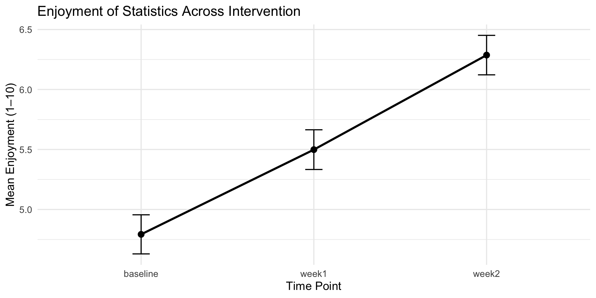
Prof. Brocker wants to evaluate whether a new engagement intervention improves students’ attitudes toward statistics. At the beginning of the semester, 100 students complete a survey rating how much they enjoy statistics on a scale from 1 (not at all) to 10 (extremely).He then implements a two-week intervention in which each class begins with a brief statistics-related warm-up activity designed to increase interest and reduce anxiety. After the first week of the intervention, students rate their enjoyment of statistics again. At the end of the second week, they complete the rating a third time.
dfTime =
dfSubjects =
dfError =
n =
Practice
Prof. Brocker wants to evaluate whether a new engagement intervention improves students’ attitudes toward statistics. At the beginning of the semester, 100 students complete a survey rating how much they enjoy statistics on a scale from 1 (not at all) to 10 (extremely).He then implements a two-week intervention in which each class begins with a brief statistics-related warm-up activity designed to increase interest and reduce anxiety. After the first week of the intervention, students rate their enjoyment of statistics again. At the end of the second week, they complete the rating a third time.
dfTime = 3 - 1 = 2
dfSubjects = 100-1 = 99
dfError = (100 - 1) * (3-1) = 198
n = 100
Practice
Prof. Brocker wants to evaluate whether a new engagement intervention improves students’ attitudes toward statistics.
Code
library(tidyverse)library(ez)library(afex)set.seed(2025) # for reproducibilityn <-100# Baseline: lower enjoyment, more variabilitybaseline <-rnorm(n, mean =4.8, sd =1.6)# After Week 1: slight increaseweek1 <- baseline +rnorm(n, mean =0.7, sd =0.5)# After Week 2: additional increaseweek2 <- week1 +rnorm(n, mean =0.8, sd =0.5)# Keep scores bounded between 1 and 10clip <-function(x) pmin(pmax(x, 1), 10)baseline <-clip(baseline)week1 <-clip(week1)week2 <-clip(week2)# Construct long datasetdata_long <-tibble(id =factor(1:n),baseline = baseline,week1 = week1,week2 = week2) %>%pivot_longer(cols = baseline:week2,names_to ="time",values_to ="enjoyment")aov_ez(data = data_long,dv ="enjoyment",id ="id",within ="time",anova_table =list(es ="ges"),return ="aov") |>tidy() |>rename(Source = term,SS = sumsq,MS = meansq,`F`= statistic, p = p.value ) |>select(-stratum) |>filter(Source =="time"| df ==198) |>gt() |>fmt_auto()
Source
df
SS
MS
F
p
time
2
111.716
55.858
343.599
4.101 × 10−65
Residuals
198
32.188
0.163
NA
NA
Code
data_long %>%group_by(time) %>%summarize(mean =mean(enjoyment), se =sd(enjoyment)/sqrt(n)) %>%ggplot(aes(x = time, y = mean, group =1)) +geom_line(size =1.2) +geom_point(size =3) +geom_errorbar(aes(ymin = mean - se, ymax = mean + se), width =0.1) +labs(title ="Enjoyment of Statistics Across Intervention",x ="Time Point",y ="Mean Enjoyment (1–10)") +theme_minimal(base_size =14)
ANOVA
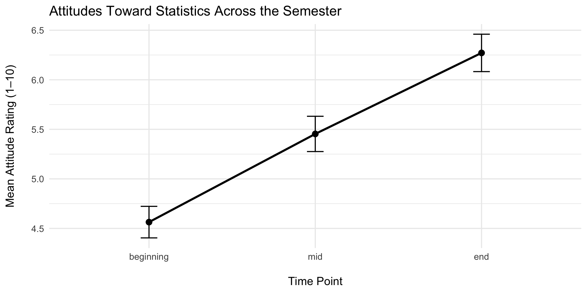
Professor Brocker is interested in whether structured active-learning practices improve 80students’ attitudes toward statistics over time. He administers a 1–10 enjoyment rating at three points:
Beginning of the semester (before any intervention).
After four active-learning modules (mid-semester).
After eight active-learning modules (end of the semester).
dfTime =
dfParticipants =
dfError =
Practice
Professor Brocker is interested in whether structured active-learning practices improve 80 students’ attitudes toward statistics over time. He administers a 1–10 enjoyment rating at three points:
Beginning of the semester (before any intervention).
After four active-learning modules (mid-semester).
After eight active-learning modules (end of the semester).
dfTime = 3 - 1 = 2
dfParticipants = 80 - 1 = 79
dfError = 158
Practice
Professor Brocker is interested in whether structured active-learning practices improve 80 students’ attitudes toward statistics over time. He administers a 1–10 enjoyment rating at three points:
Code
set.seed(2025)n <-80# Attitude ratings (1–10 scale)beginning <-rnorm(n, mean =4.5, sd =1.4) # before any modulesmid <- beginning +rnorm(n, mean =1.0, sd =0.6) # after 4 modulesend <- mid +rnorm(n, mean =0.8, sd =0.5) # after 8 modules# Bound values between 1 and 10clip <-function(x) pmin(pmax(x, 1), 10)beginning <-clip(beginning)mid <-clip(mid)end <-clip(end)# Create long datasetdata_long2 <-tibble(id =factor(1:n),beginning = beginning,mid = mid,end = end) |>pivot_longer(cols = beginning:end,names_to ="time",values_to ="attitude" ) |>mutate(time =factor(time, levels =c("beginning","mid","end")) )# ------------------------------# Repeated-Measures ANOVA# ------------------------------rm_aov <-aov_ez(id ="id",dv ="attitude",within ="time",data = data_long2,anova_table =list(es ="ges"),return ="aov")# Clean table for displayrm_aov |>tidy() |>rename(Source = term,SS = sumsq,MS = meansq,`F`= statistic, p = p.value ) |>select(!stratum) |>gt()
Source
df
SS
MS
F
p
Residuals
79
552.89748
6.998702
NA
NA
time
2
116.75497
58.377487
281.961
7.467537e-53
Residuals
158
32.71248
0.207041
NA
NA
Code
data_long2 |>group_by(time) |>summarize(mean =mean(attitude),se =sd(attitude) /sqrt(n) ) |>ggplot(aes(fct_inorder(time, ordered =TRUE), mean, group =1)) +geom_line(size =1.2) +geom_point(size =3) +geom_errorbar(aes(ymin = mean - se, ymax = mean + se), width =0.1) +labs(title ="Attitudes Toward Statistics Across the Semester",x ="\nTime Point",y ="Mean Attitude Rating (1–10)\n" ) +theme_minimal(base_size =14)
Practice
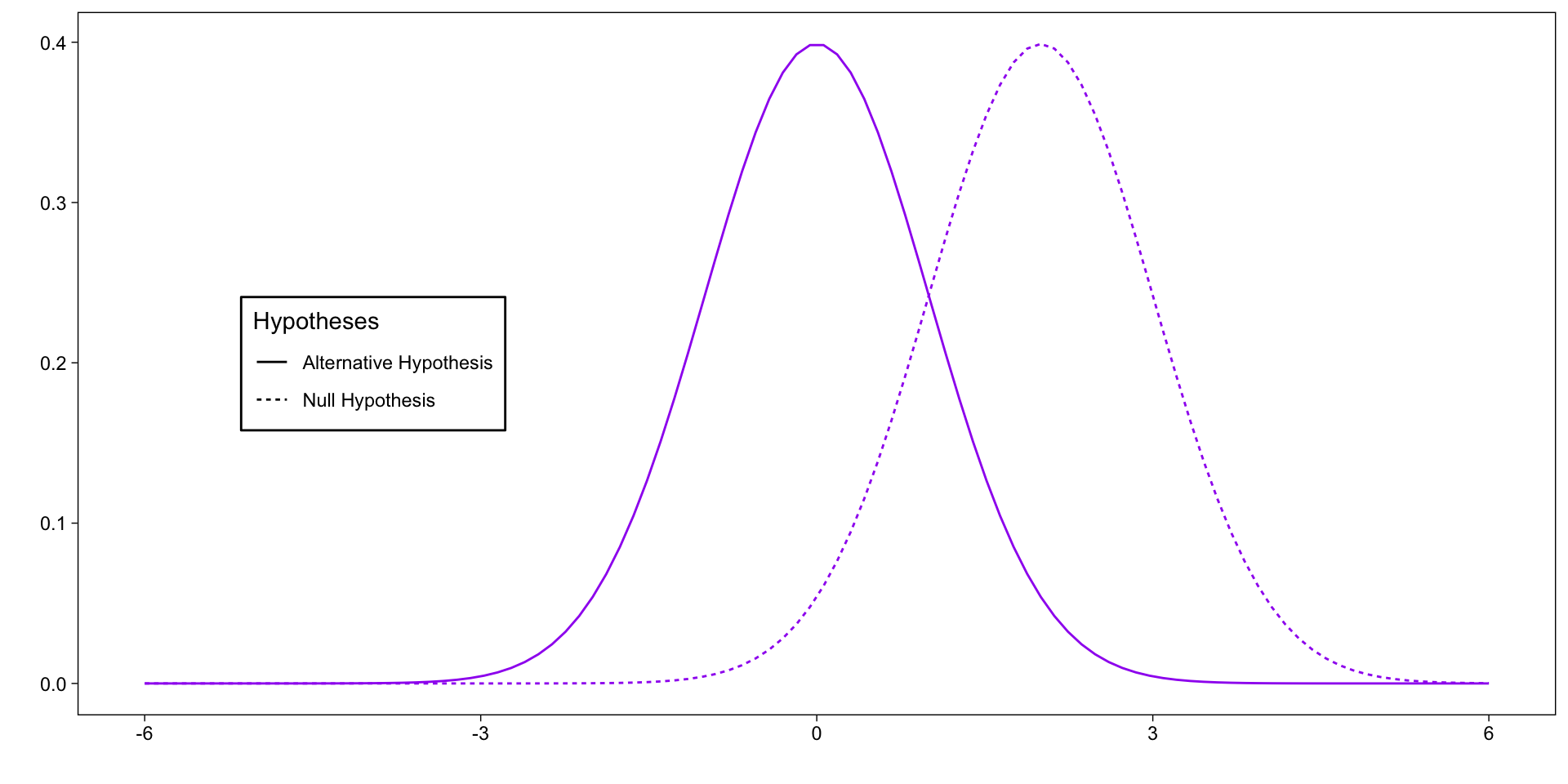
Interpreting F
MSTime is made up of MSError + the theoretical difference over time:
\(MS_{Time} = \text{change over time} + MS_{Error}\)
\(MS_{Time} = 0 + MS_{Error}\)
\(MS_{Time} = MS_{Error}\)
\(F = \frac{MS_{Error}}{MS_{Error}} = 1\)
Interpreting F
When F <= 1, it’s not likely to be significant.
The MSTime is made up of the MSError + the theoretical difference over time:
\(MS_{Time} = \text{change over time} + MS_{Error}\)
\(MS_{Time} = \text{effect} + MS_{Error}\)
\(F > 1\)
Hypothesis testing: ANOVA
\(F \leq 1\)
Fail to reject the Null Hypothesis
\(F > 1\)
Refer to p-value
Reject the Null Hypothesis
Reporting F
If asked to report findings in terms of the Null Hypothesis (H0), you should report findings as:
Reject H0, or
Fail to Reject H0
If asked to report findings in general or for publication, you need to report:
\(F(df_{Time}, df_{Error}) = F, p\)
Reporting F
Enjoyment of statistics after three weeks was significantly higher compared to enjoyment of statistics at the start of measurement, F (2, 158) = 281.96, p <.001
If the results are significant, we have to also report the means and standard deviations for each time point.
Participants’ enjoyment of statistics differed significant across time, F(2, 158) = 281.96, p <.001. Enjoyment was highest at week 2 (M= 6.61, s = 1.77). Enjoyment was lowest at baseline (M = 5.14, s = 1.62). Anxiety at week 1 test was M= 5.86, s = 1.67.
Data Manipulation
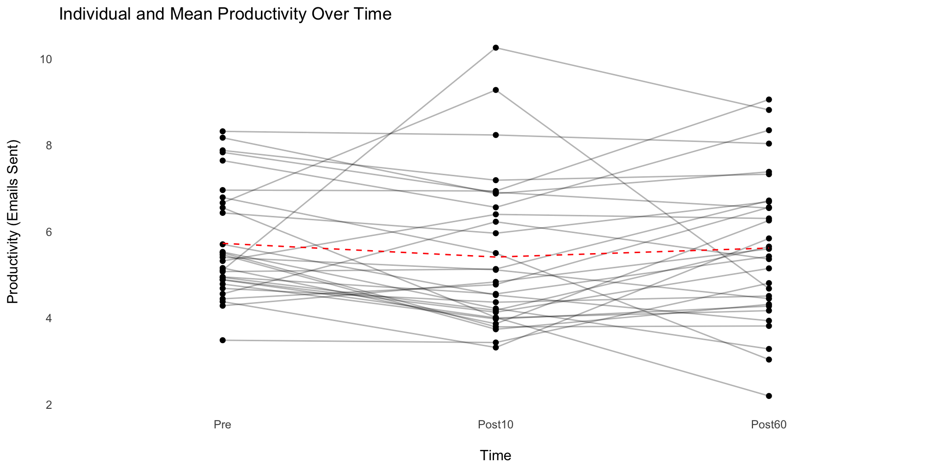
When collected, data can be in either wide or long format.
Below are the first five rows of the same dataset:
Code
data.frame(Participant =factor(1:5),Immediate =rnorm(5, mean =8, sd =1.5),After24Hours =rnorm(5, mean =6, sd =1.5),After1Week =rnorm(5, mean =4, sd =1.5)) |>gt() |>tab_header(title ="Wide Data",subtitle ="Each row represents an indivdual participant")
Wide Data
Each row represents an indivdual participant
Participant
Immediate
After24Hours
After1Week
1
8.705734
5.686030
5.851281
2
6.397846
7.113822
3.414249
3
5.571551
8.255040
4.175469
4
6.417572
5.461643
2.616414
5
6.597311
4.543876
2.219887
Code
data.frame(Participant =factor(1:5),Immediate =rnorm(5, mean =8, sd =1.5),Day =rnorm(5, mean =6, sd =1.5),Week =rnorm(5, mean =4, sd =1.5)) |> tidyr::pivot_longer(cols =!Participant,names_to ="Time",values_to ="Stress") |>gt() |>fmt_auto() |>tab_header(title ="Long Data",subtitle ="Each row represents an indivdual participant's score on each level of the treatment")
Long Data
Each row represents an indivdual participant's score on each level of the treatment
Participant
Time
Stress
1
Immediate
6.566
1
Day
6.58
1
Week
1.127
2
Immediate
7.219
2
Day
7.573
2
Week
3.645
3
Immediate
8.333
3
Day
7.335
3
Week
1.699
4
Immediate
9.193
4
Day
6.733
4
Week
2.172
5
Immediate
8.013
5
Day
7.256
5
Week
4.629
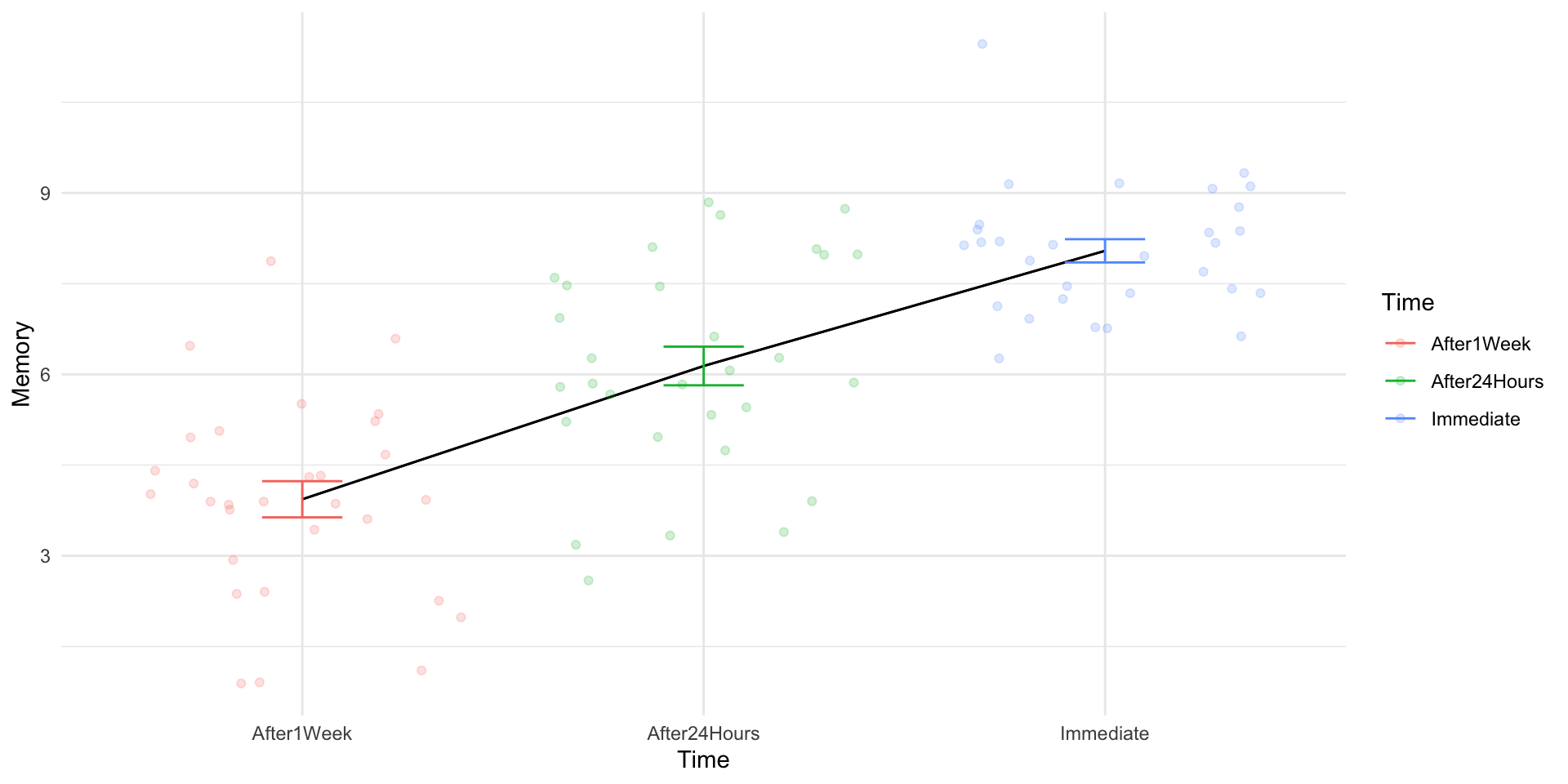
Memory Recall Study
Code
set.seed(100)# Memory Recall Studymemory_data <-data.frame(Participant =factor(1:30),Immediate =rnorm(30, mean =8, sd =1.5),After24Hours =rnorm(30, mean =6, sd =1.5),After1Week =rnorm(30, mean =4, sd =1.5))# Make Data Longermemory_data_long <- memory_data |>pivot_longer(cols =!Participant,names_to ="Time",values_to ="Memory")aov(Memory ~ Time +Error(Participant), data = memory_data_long) |>tidy() |>mutate(Source = term,SS = sumsq,MS = meansq,`F`=ifelse(is.na(statistic),"--",statistic |>round(3)),p =ifelse(p.value >.05,"<.05",p.value),p =ifelse(is.na(p),"--",p) ) |>select(Source, df, SS, MS, `F`, p) |>gt() |>fmt_auto()