Factorial ANOVA
PSY 348: Lecture 13
Dave Brocker
Farmingdale State College
What is a Factorial ANOVA?
More than 1 independent variable
- Up to now, we’ve looked at experiments that test one question at a time.
t-test
Do two groups differ?
“Does drinking coffee make people happier than not drinking coffee?”
One-way ANOVA
Do more than two groups differ on one IV?
“Does coffee make people happier, compared to decaf or water?”
- But in real life, there’s rarely just one thing influencing behavior.
Why Factorial ANOVA?
A Factorial ANOVA allows us to test more than one independent variable (IV) at the same time.
Instead of asking separate questions:
“Does coffee make people happier?”
“Does watching TV make people happier?”
We can now ask:
“Does coffee and watching TV make people happier?”
“Does the effect of coffee depend on what you’re watching?”
The Power of Two (or More)
Testing as separate IVs
The Power of Two (or More)
Combining IVs
The Power of Two (or More)
Three questions at once
- Main Effect 1
- Does IV1 alone affect the outcome? (Coffee → Happiness)
- Main Effect 2
- Does IV2 alone affect the outcome? (TV Show → Happiness)
- Interaction Effect
- Does the effect of one variable depend on the other? (Maybe coffee only helps if you’re watching TV!)
Why Not Just Run Multiple t-tests?
You could compare…
Coffee vs. No Coffee
Dark vs. No Dark
Coffee + Dark vs. everything else
- but each additional t-test increases your Type I error rate (false positives).
A Factorial ANOVA solves that problem by testing all these relationships in one model, controlling for shared variance and examining combined effects.
In Other Words…
| Test Type | Question | Example |
|---|---|---|
| t-test | Do two groups differ? | Coffee vs. No Coffee |
| One-Way ANOVA | Do 3+ groups differ on one IV? | Decaf, Coffee, Energy Drink |
| Factorial ANOVA | How do two or more IVs work together? | Coffee × TV Show → Happiness |
The Goal of Research
The goal of good research is to narrow in on the real sources of variation.
Factorial ANOVA lets us see not just whether variables matter, but how they matter together.
It’s not just what causes an effect, it’s what combinations of causes create patterns we care about.
Factorial ANOVA
Four sources of variance
- Between IV 1
- Variance between the groups of the first IV (main effect 1).
- Between IV 2
- Variance between the groups of the second IV (main effect 2).
- Interaction
- Variance from the combination of the groups (the cells).
- Error
- Variance within each cell, around that cell’s own mean.
Understanding Main Effects
The main effect of Coffee asks:
- On average, does drinking coffee make people happier than not drinking coffee?
(Regardless of whether they watched TV or not.)
- On average, does drinking coffee make people happier than not drinking coffee?
The main effect of Watching TV asks:
- On average, does watching TV make people happier than not watching it?
(Regardless of whether they had coffee or not.)
- On average, does watching TV make people happier than not watching it?
Understanding Main Effects
The 2 × 2 table of means
| 2 × 2 Factorial Design: Coffee × TV | ||
| Mean happiness by condition (cell means) | ||
| Watched TV? |
Coffee condition
|
|
|---|---|---|
| Coffee | No Coffee | |
| TV | 3.0 | 4.0 |
| No TV | 4.0 | 8.0 |
| With marginal means | |||
| Row and column means show the main effects | |||
| Watched TV? | Coffee | No Coffee | Row mean |
|---|---|---|---|
| TV | 3.0 | 4.0 | 3.5 |
| No TV | 4.0 | 8.0 | 6.0 |
| Column mean | 3.5 | 6.0 | 4.8 |
Coffee main effect: 3.50 (coffee) vs. 6.00 (no coffee).
TV main effect: 3.50 (TV) vs. 6.00 (no TV).
Visualizing Interactions
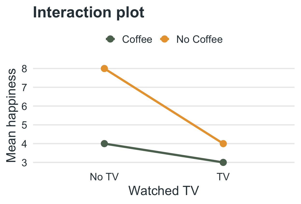
Each line is one level of the first IV (coffee). The x-axis is the second IV (TV).
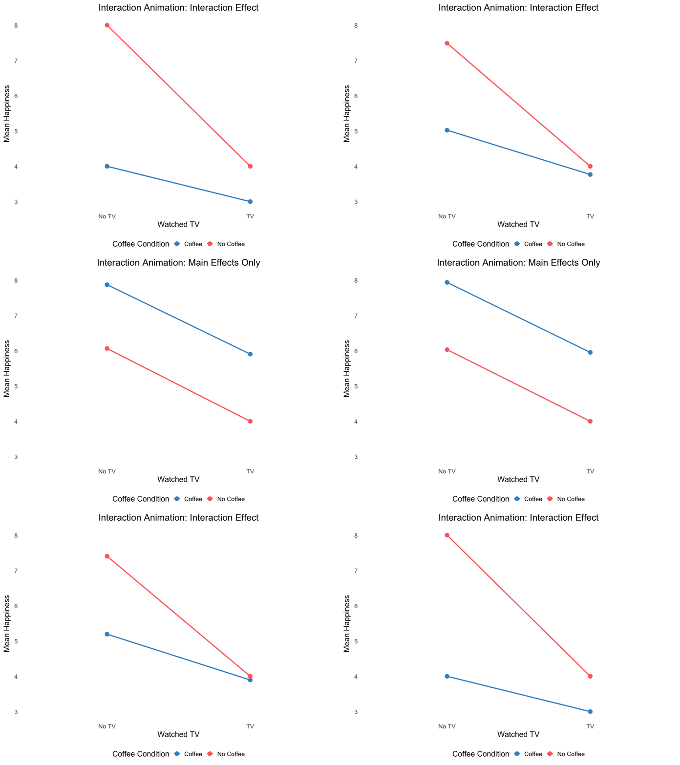
Parallel lines mean no interaction: the effect of one IV doesn’t depend on the other.
Here the lines are not parallel. Without coffee, TV drops happiness a lot (8.00 to 4.00). With coffee, TV matters much less (4.00 to 3.00). That is an interaction.
Visualizing Interactions
A main effect hides the story
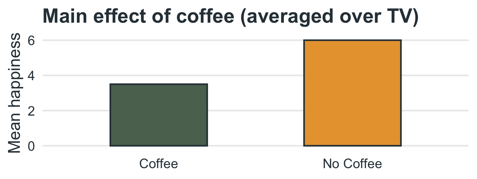
- Averaged over TV, coffee drinkers are less happy (3.50 vs. 6.00). The interaction plot shows the full story: the size of the difference depends on whether people watched TV.
Visualizing Interactions
From main effect to interaction
Calculating F Values
Degrees of freedom
Between groups 1: \(df_{B_1} = k_1 - 1\)
Between groups 2: \(df_{B_2} = k_2 - 1\)
Interaction: \(df_{Interaction} = (k_1 - 1) \times (k_2 - 1)\)
Error: \(df_{Error} = N - (k_1 \times k_2)\)
Total: \(df_{Total} = N - 1\)
Calculating MS
Each MS is an SS divided by its df
\(MS_{B_1} = \dfrac{SS_{B_1}}{k_1-1} \qquad MS_{B_2} = \dfrac{SS_{B_2}}{k_2-1}\)
\(MS_{Interaction} = \dfrac{SS_{Interaction}}{(k_1-1)(k_2-1)} \qquad MS_{Error} = \dfrac{SS_{Error}}{N-(k_1 k_2)}\)
- Each SS is a sum of squared distances from a mean: \(SS_{B_1} = \sum n_j(\bar{x}_j - \bar{x}_G)^2\) (each level mean from the grand mean, weighted by group size; same form for \(SS_{B_2}\)) and \(SS_{Error} = \sum (x - \bar{x}_{cell})^2\) (each score from its own cell mean). \(SS_{Interaction}\) is what remains of the between-cell variation after \(SS_{B_1}\) and \(SS_{B_2}\).
Calculating F
Every F uses the same denominator
\(F_A = \dfrac{MS_{B_1}}{MS_{Error}} \qquad F_B = \dfrac{MS_{B_2}}{MS_{Error}} \qquad F_{AB} = \dfrac{MS_{Interaction}}{MS_{Error}}\)
How Many F’s?
Factorial ANOVA in R
The model formula
factorial_anova.R
                           Df Sum Sq Mean Sq F value   Pr(>F)
diet_type                   1 101.27  101.27  41.899 4.06e-09 ***
exercise_regimen            1 114.06  114.06  47.191 6.41e-10 ***
diet_type:exercise_regimen  1   9.07    9.07   3.751   0.0557 .
Residuals                  96 232.02    2.42
---
Signif. codes:  0 '***' 0.001 '**' 0.01 '*' 0.05 '.' 0.1 ' ' 1
diet_type * exercise_regimenis shorthand fordiet_type + exercise_regimen + diet_type:exercise_regimen.Each row of the table is one F-test: two main effects and the interaction.
Interpreting Results
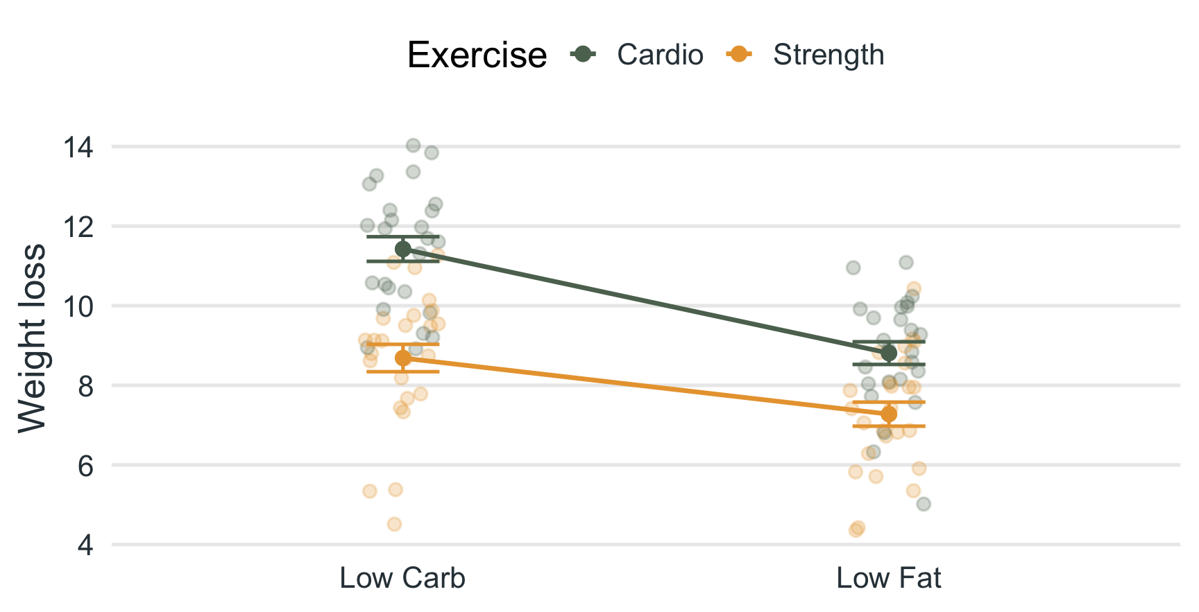
Example 1: weight loss, diet type × exercise regimen
Interpreting the Fs in 2-way ANOVA
\(F_A\) (Diet type): F(1, 96) = 41.90, p < .001
\(F_B\) (Exercise regimen): F(1, 96) = 47.19, p < .001
\(F_{AB}\) (Diet × Exercise): F(1, 96) = 3.75, p = .056 (not significant)
Both main effects are significant and the interaction is not, so the effect of diet is about the same at each exercise regimen (and vice versa): the lines in the plot are close to parallel.
Interpreting Results
Example 2: political interest, gender × education
| Source | df | SS | MS | F | p |
|---|---|---|---|---|---|
| gender | 1 | 216.57 | 216.57 | 244.15 | <.001 |
| education_level | 3 | 198.31 | 66.10 | 74.52 | <.001 |
| gender:education_level | 3 | 23.65 | 7.88 | 8.89 | <.001 |
| Residuals | 92 | 81.61 | 0.89 | – | – |
| Dependent Variable: Political Interest Gender: Male, Female Education: High School, Bachelor’s, Master’s, PhD |
|||||
Gender: F(1, 92) = 244.15, p < .001
Education: F(3, 92) = 74.52, p < .001
Gender × Education: F(3, 92) = 8.89, p < .001
Interpreting F’s
Visually
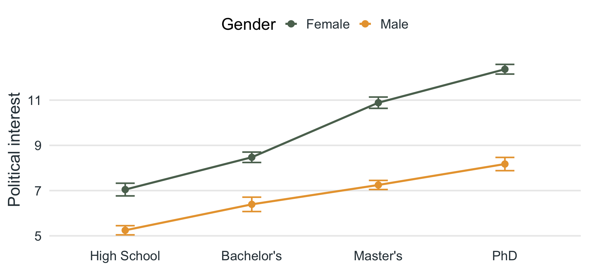
- The lines are not parallel: the effect of education depends on gender, which is why the interaction is significant.
Effect Size: Partial Eta Squared
\(\eta_p^2\)
\(\eta_p^2 = \dfrac{SS_{effect}}{SS_{effect} + SS_{error}}\) (one value for each F)
- Numerator: the SS for this effect. Denominator: that same SS plus the error SS.
| Effect | Partial η² |
|---|---|
| Diet type | 0.304 |
| Exercise regimen | 0.330 |
| Diet × Exercise | 0.038 |
- Benchmarks are the same as one-way ANOVA: about .01 small, .06 medium, .14 large.
Following Up an Interaction
What if the interaction is significant?
A significant interaction means the effect of one IV depends on the other, so interpret the cells, not just the main effects.
Compare the cell means with a post-hoc test, or test the effect of one IV at each level of the other (simple effects).
follow_up.R
- In the weight-loss example the interaction was not significant, so we interpret the two main effects.
Assumptions of Factorial ANOVA
Assumptions
- The DV is continuous (interval or ratio scale).
- Observations are independent. Each person is in only one cell.
- Normality: scores (residuals) are approximately normal in each cell.
- Homogeneity of variance: the cells have similar variances (Levene’s Test).
Reporting F
If asked to report findings in terms of the Null Hypothesis (H0), you should report findings as:
Reject \(H_0\), or
Fail to Reject \(H_0\)
Reporting F
If asked to report findings in general or for publication, you need EACH F-value:
\(F\)(df between, df error) = F-value
the corresponding p-value
an effect size (\(\eta_p^2\))
for significant results: the means and standard deviations of each group
Reporting F
Main effect of diet type
Participants on the low-carb diet (M = 10.06, SD = 2.13) lost significantly more weight than participants on the low-fat diet (M = 8.04, SD = 1.65), F(1, 96) = 41.90, p < .001, \(\eta_p^2\) = 0.30.
Reporting F
Main effect of exercise regimen
Participants who did cardio (M = 10.12, SD = 1.98) lost significantly more weight than participants who did strength training (M = 7.98, SD = 1.75), F(1, 96) = 47.19, p < .001, \(\eta_p^2\) = 0.33.
Reporting F
Interaction
If NOT significant: The interaction between diet type and exercise regimen was not significant, F(1, 96) = 3.75, p = .056.
If significant: report the cell means and standard deviations, and describe the pattern (e.g., “the benefit of cardio was larger for the low-carb diet”).
Factorial ANOVA Wrap-Up
Connecting the dots
Big picture: a factorial ANOVA lets us test multiple independent variables at once.
- Not just whether each matters, but whether they matter together.
Understanding Interactions
What it tests
| Source | Question | Interpretation |
|---|---|---|
| Main Effect A | Does IV1 (e.g., Coffee) affect the DV on average? | “Coffee drinkers happier?” |
| Main Effect B | Does IV2 (e.g., TV Show) affect the DV on average? | “TV watchers happier?” |
| Interaction (A × B) | Does the effect of Coffee depend on watching TV? | “Coffee only helps if watching TV?” |
Factorial ANOVA | ⬡⬢⬡⬢⬡⬢