ANOVA compares the means of different groups to determine if they differ significantly from one another.
ANOVA can examine independent variables with more than 2 groups.
ANOVA can also look at multiple independent variables.
2-way AnOVA
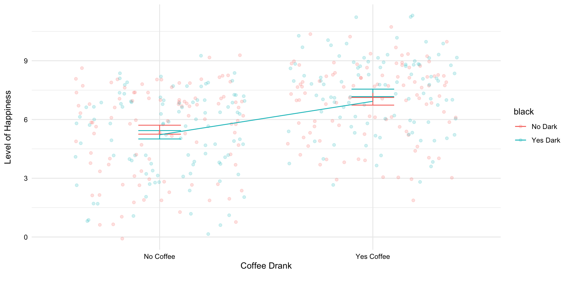
Prof Brocker believes the key to happiness involves 2 things: drinking coffee and Dark. He wants to see if drinking coffee makes participants significantly happier than not drinking coffee. He also wants to see if watching Dark show makes them significantly happier than not watching it.
What kind of design is he using?
2 x 2
2-way AnOVA
We can write the design of a study analyzed using ANOVA as:
Number of groups “x” the Number of groups
Conditions in the first independent variable “x” Conditions in the second independent variable, etc.
2 x 2
2-way AnOVA
Prof Brocker believes the key to happiness involves 2 things: coffee and Dark. He wants to see if drinking coffee makes participants significantly happier than not drinking coffee. He also wants to see if watching Dark show makes them significantly happier than not watching it. This is a 2 x 2 design.
IV1 = Number of groups in coffee: 2 (coffee or no coffee)
IV2 = Number of groups in Dark: 2 (Dark or No Dark)
DV
Happiness
2-way Anova
What are Prof Brocker’s Alternative Hypotheses?
H1: Participants who drink coffee will be significantly happier than those who don’t.
H2: Participants who watch Dark will be significantly happier than those who don’t.
2-way AnOVA
Prof Brocker believes the key to happiness involves 2 things: coffee and Dark. He wants to see if drinking coffee makes participants significantly happier than not drinking coffee. He also wants to see if watching Dark show makes them significantly happier than not watching it. This is a 2 x 2 design.
Participants who drink coffee will be significantly happier than those who don’t.
Participants who watch Dark will be significantly happier than those who don’t.
H3: Participants who drink coffee while watching the Dark will be the happiest.
ANOVA
The Three Types
Between-subjects: [One-Way or Factorial]
Within-subjects: (Repeated Measures ANOVA)
Mixed-designs: Combination of Between and Within
2-way Between subjects ANOVA
IVs must be nominal/categorical
DV must be continuous
2-way Between subjects ANOVA
IVs must be nominal/categorical
DV must be continuous
2-way ANOVA
Two types of variance:
Variance among all of the scores (error variance).
Variance between the groups of the first IV (between group variance 1).
Variance between the groups of the second IV (between group variance 2).
Variance between the combination of the groups (interaction variance).
2-way ANOVA
Code
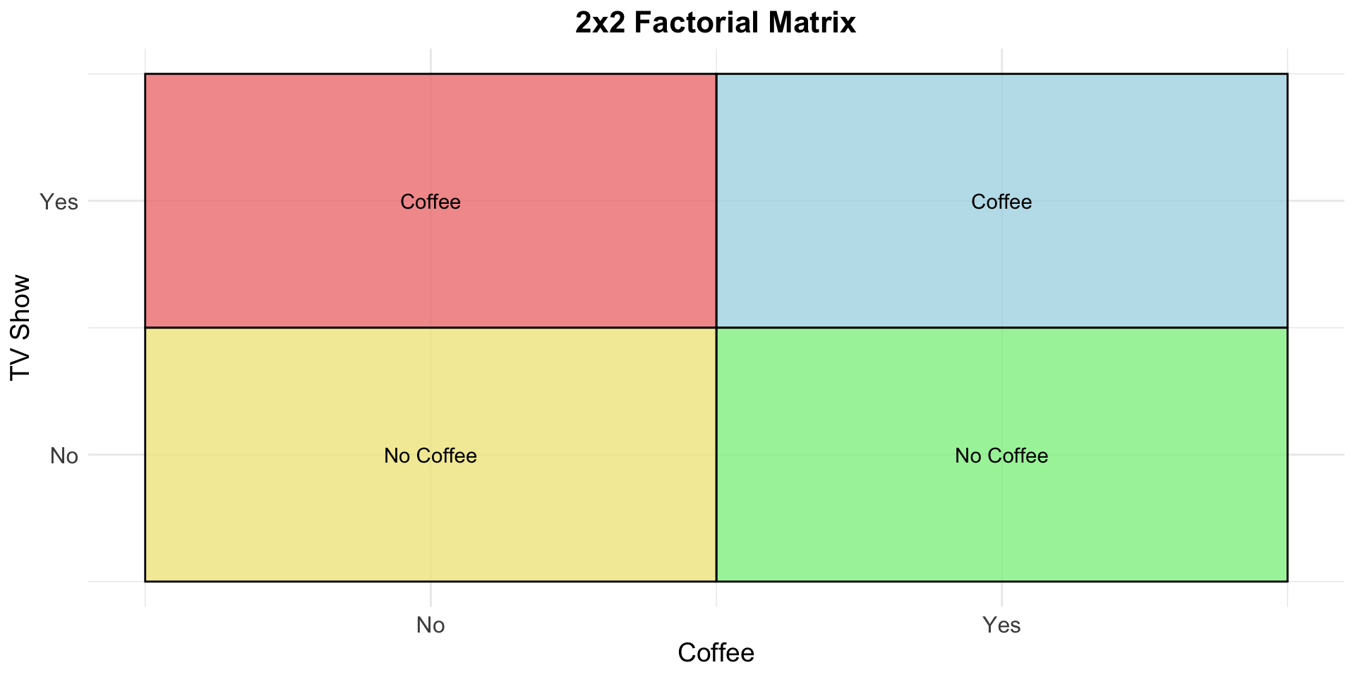
# Load librarieslibrary(dplyr)library(ggplot2)library(gt)library(broom)# Create a 2x2 grid structure for visualizationmatrix_data <-expand.grid(Coffee =c("Yes", "No"),TV_Show =c("Yes", "No")) %>%mutate(x =as.numeric(Coffee =="Yes"),y =as.numeric(TV_Show =="Yes"),fill_color =c("lightblue", "lightcoral", "lightgreen", "khaki") # Assign colors )# Visualize the 2x2 matrixfac_mat <-ggplot(matrix_data, aes(xmin = x -0.5, xmax = x +0.5, ymin = y -0.5, ymax = y +0.5)) +geom_rect(aes(fill = fill_color), color ="black", alpha =0.8) +# Draw rectanglesscale_fill_identity() +# Use fill_color directlylabs(title ="2x2 Factorial Matrix",x ="Coffee", y ="TV Show" ) +scale_x_continuous(breaks =c(0, 1), labels =c("No", "Yes"), limits =c(-0.5, 1.5)) +scale_y_continuous(breaks =c(0, 1), labels =c("No", "Yes"), limits =c(-0.5, 1.5)) +theme_minimal() +theme(axis.text =element_text(size =12),axis.title =element_text(size =14),plot.title =element_text(size =16, face ="bold", hjust =0.5) )
2-way ANOVA
Code
fac_mat +annotate("text", x =1, y =1, label ="Coffee" ) +annotate("text", x =0, y =1, label ="Coffee" ) +annotate("text", x =0, y =0, label ="No Coffee" ) +annotate("text", x =1, y =0, label ="No Coffee" )
2-way ANOVA
Code
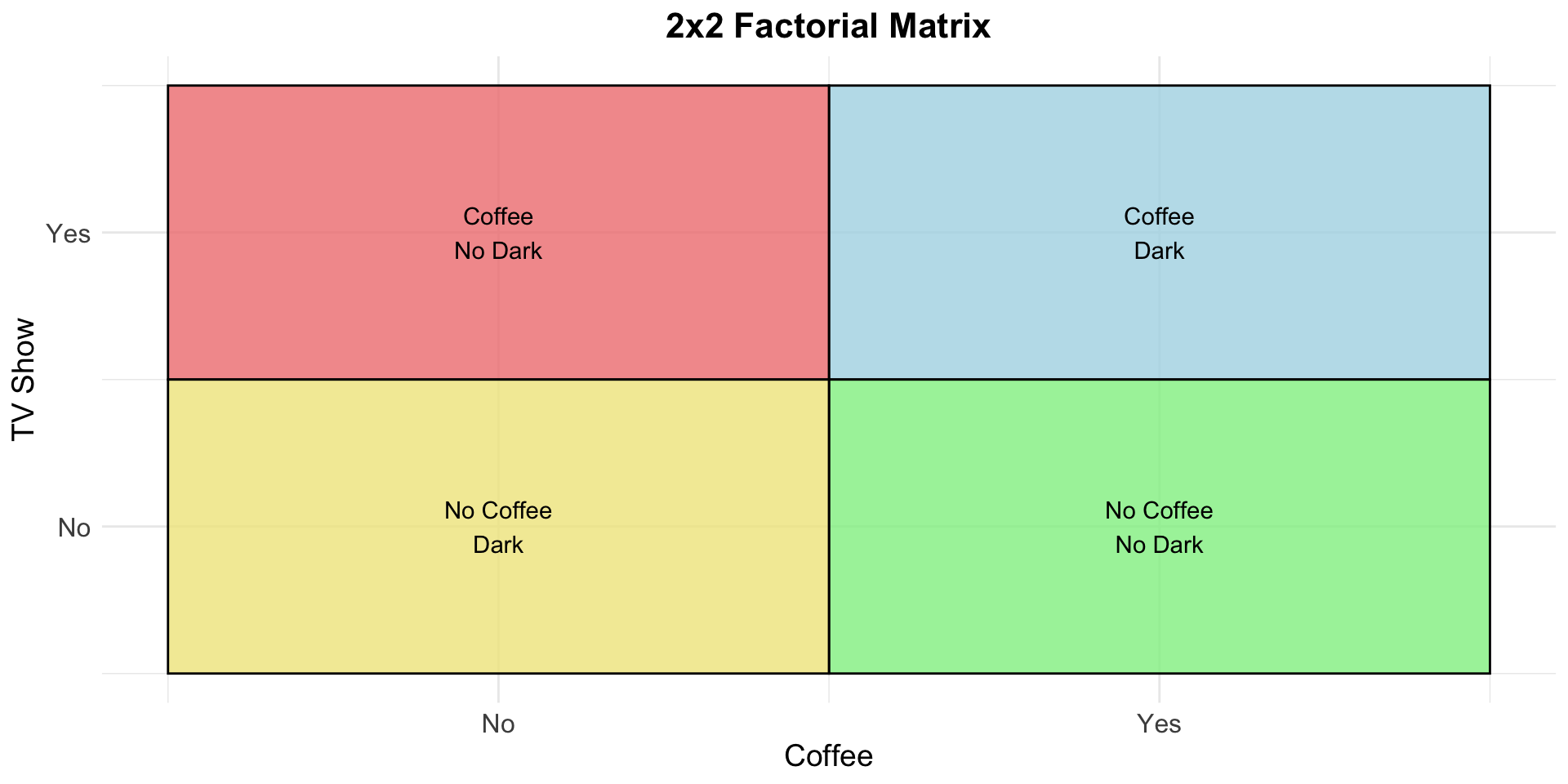
fac_mat +annotate("text", x =1, y =1, label ="Coffee\nDark" ) +annotate("text", x =0, y =1, label ="Coffee\nNo Dark" ) +annotate("text", x =0, y =0, label ="No Coffee\nDark" ) +annotate("text", x =1, y =0, label ="No Coffee\nNo Dark" )
2-way ANOVA
To compare the means, we analyzing two types of variance:
Variance among all of the scores (within group variance).
Variance between the groups of the first IV (between group variance 1).
Variance between the groups of the second IV (between group variance 2).
Variance between the combination of the groups (interaction variance).
Calculating the Fs
Degrees of freedom
The number of observations (data points) in the data that are free to vary when estimating a statistic.
I own 7 pairs of sock. I want to wear a different pair of socks every day.
How many times do I get to pick a pair of socks before I get stuck?
The degrees of freedom is how many times things can vary before we are stuck with what’s left over.
Degrees of freedom
Between Groups (dfBG ) = number of groups (k) - 1
Error Groups (dfError) = number of participants (n) - number of groups (k)
dfTotal = n - 1
*k is the number of groups in the independent variable.
Degrees of freedom
Between Groups 1 (dfBG1 ) = k1 - 1
Between Groups 2 (dfBG2 ) = k2 - 1
Interaction (MSInteractioni) = (k1 - 1) x (k2 - 1)
Error (MSError) = n - (k1 x k2)
Total = n - 1
*k is the number of groups in each independent variable.
Prof Brocker believes the key to happiness involves 2 things: Coffee and Dark. He wants to see if drinking coffee makes participants significantly happier than not drinking coffee. He also wants to see if watching Dark show makes them significantly happier than not watching it. This is a 2 x 2 design.
He randomly assigns 100 participants to Coffee and Dark or No Coffee x Dark or NoCoffee and No Dark.
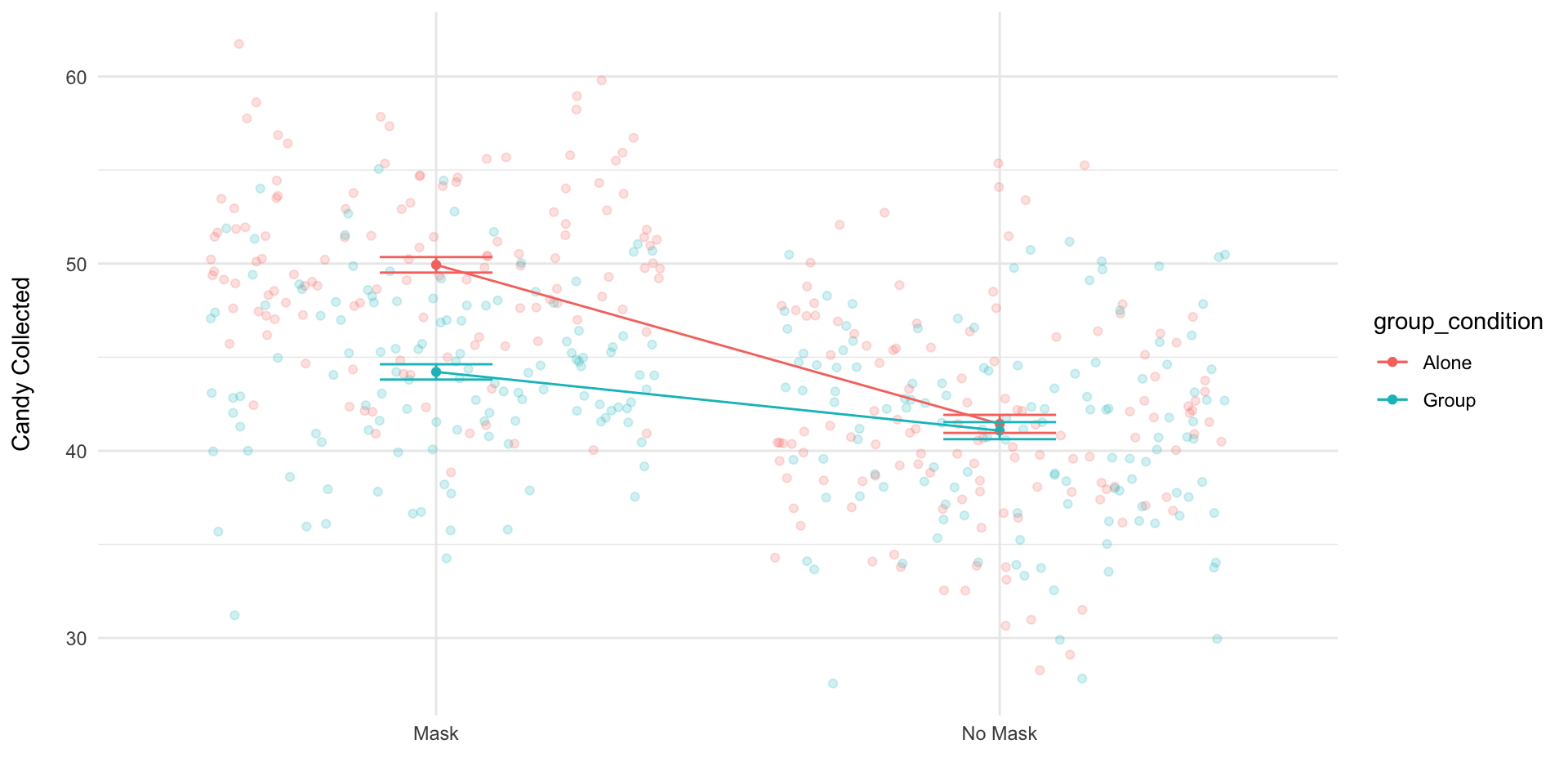
Prof. Brocker recruit 500 children on Halloween. He assigns half to wear a costume with a mask, and the other half to wear a costume without a mask. He assigns participants to trick-or-treat alone or in groups. Then he measures how much candy each child collects while trick-or-treating.
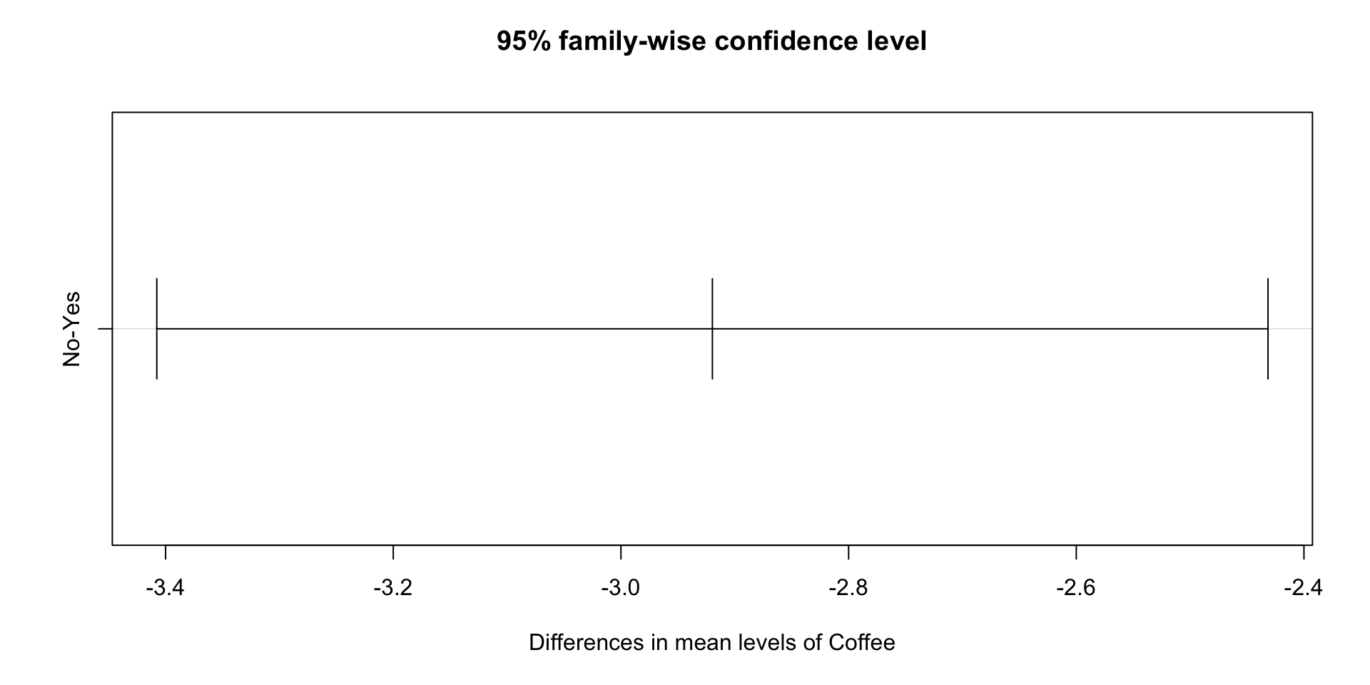
If asked to report findings in terms of the Null Hypothesis (H0), you should report findings as:
Reject H0, or
Fail to Reject H0
Reporting F
If asked to report findings in general or for publication, you need EACH F-value:
F(dfBG, dfW )
= F-value
Corresponding p-value
For significant results: Means and standard deviations of each group
Reporting F
The group that watched Dark (M=8.43, s=1.02) reported significantly more happiness compared to their peers in the control group who watched Jeopardy (M=6.12, s=0.98), F(1,496) = 7.12, p < 0.05.
Reporting F
Results IV1:
If significant: The group that watched Dark (M=8.43, s=1.02) reported significantly more happiness compared to their peers in the control group who watched Jeopardy (M=6.12, s=0.98), F (1, 496) = 7.12, p < 0.05.
If NOT significant: There was not a significant difference in happiness between the groups, F (1, 498) = 1.02, p = 0.07.
Reporting F
Results IV2:
If significant: The group that drank coffee (M=7.35, s=1.01) reported significantly more happiness compared to their peers in the control group who drank decaf (M=4.21, s=0.99), F (1, 496) = 9.12, p < 0.05.
If NOT significant: There was not a significant difference in happiness between the groups, F (1, 498) = 1.02, p = 0.07.
Reporting F
Results Interaction:
If significant: The group that drank coffee AND watched Dark (M=7.35, s=1.01) reported significantly more happiness compared to the other groups (M=4.21, s=0.99), F (1, 496) = 11.14, p < 0.05.
If NOT significant: There was not a significant difference in happiness between the groups, F (1, 498) = 1.02, p = 0.07.
Code
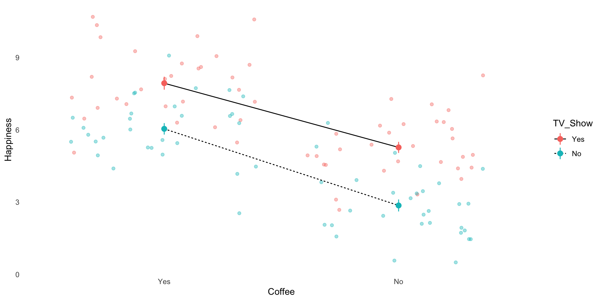
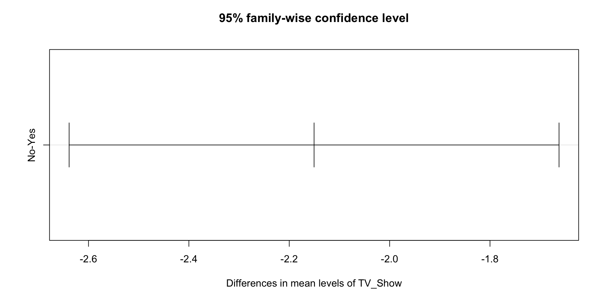
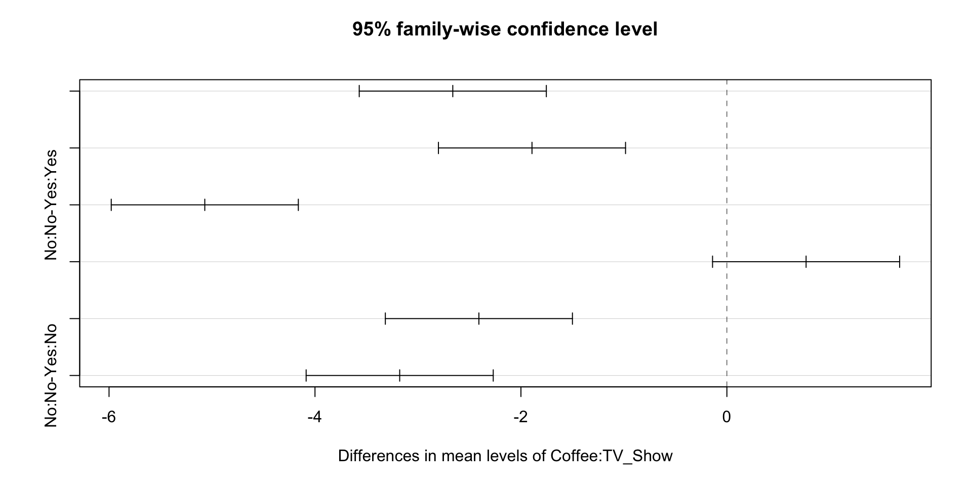
library(dplyr)library(ggplot2)# Set seed for reproducibilityset.seed(123)# Create levels for the independent variablescoffee <-c("Yes", "No")tv_show <-c("Yes", "No")# Create a data frame with all combinations of coffee and tv_showfactorial_design <-expand.grid(Coffee = coffee, TV_Show = tv_show)# Simulate happiness scores for each group# Adjust means to reflect interaction effectsn_per_group <-30# Number of participants per conditiondata <- factorial_design[rep(1:nrow(factorial_design), each = n_per_group), ]data$Happiness <-NA# Define mean happiness scores for each conditionmeans <-c("Yes_Yes"=8, # Coffee + TV Show"Yes_No"=6, # Coffee + No TV Show"No_Yes"=5, # No Coffee + TV Show"No_No"=3# No Coffee + No TV Show)# Assign happiness scores with some random noisedata$Happiness <-rnorm(n =nrow(data),mean = means[paste(data$Coffee, data$TV_Show, sep ="_")],sd =1.5# Standard deviation for noise)# Modelfac_mod <-aov(Happiness ~ Coffee * TV_Show, data = data)data |>ggplot(aes(Coffee, Happiness, color = TV_Show)) +geom_jitter(alpha = .4) +stat_summary(fun.data ="mean_se",geom ="line",color ="black",aes(group = TV_Show,lty = TV_Show) ) +stat_summary(fun.data ="mean_se",geom ="pointrange",aes(color = TV_Show) ) +theme_minimal() +theme(panel.grid =element_blank() )