Lecture 12
Farmingdale State College
The test statistic is calculated as:
\[ t = \frac{\bar{X} - \mu}{s / \sqrt{n}} \]
Where:
\(\bar{X}\) = sample mean
\(\mu\) = population mean (null hypothesis value)
\(s\) = sample standard deviation
\(n\) = sample size
\[ t = \frac{78 - 75}{5 / \sqrt{20}} = \frac{3}{1.118} = 2.68 \]
APA-style:
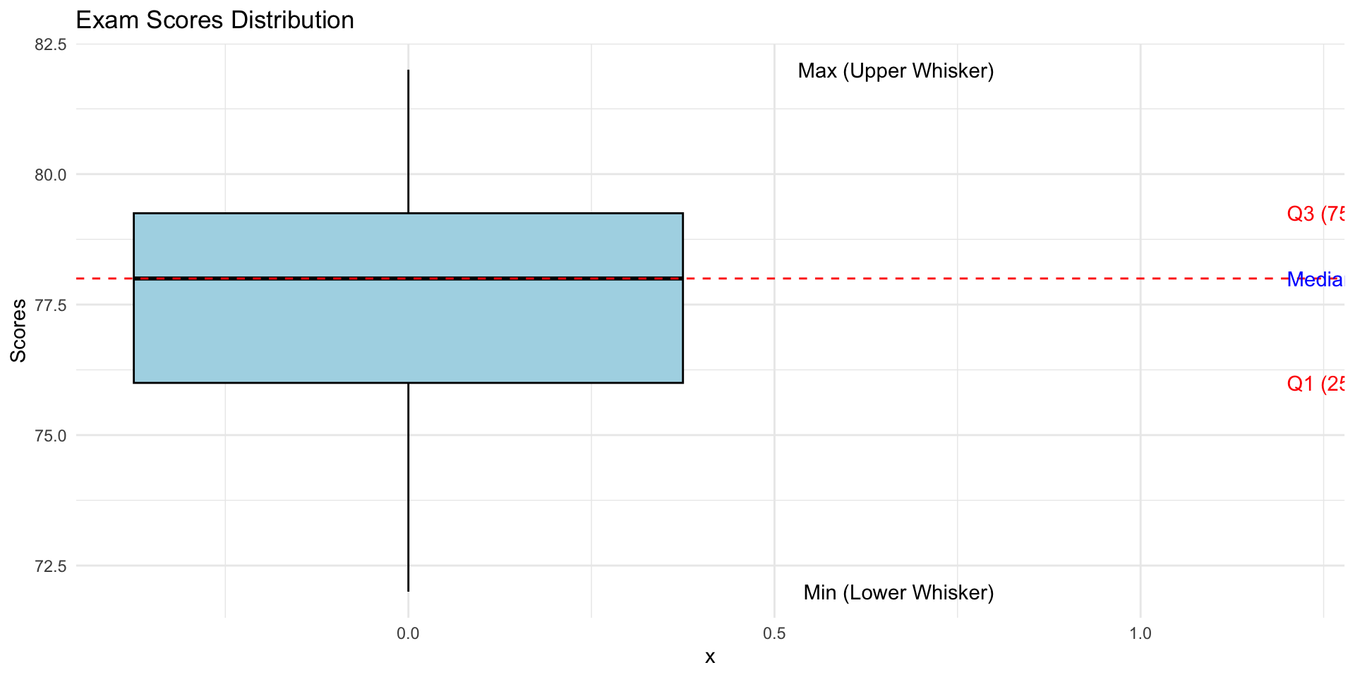
A one-sample t-test was conducted to compare exam scores to the national average of 75. Results showed a significant difference, t(19) = 2.68, p < .05, indicating that students scored significantly higher than the national average.
| Measure | Value |
|---|---|
| Sample Mean | 78 |
| Population Mean | 75 |
| Sample SD | 5 |
| Sample Size | 20 |
| t-Statistic | 2.68 |
| p-Value | 0.014 |
A professor wants to test if students in their class scored differently from the national average of 75 on an exam. A sample of 25 students has a mean score of 78 with a standard deviation of 10.
Using the one-sample t-test formula:
[ t = ]
Substituting values:
[ t = = = 1.5 ]
For df = 24, the critical value at α = .05 (two-tailed) is ±2.064. Since 1.5 < 2.064, we fail to reject (H_0).
A one-sample t-test was conducted to determine whether students’ exam scores differed from the national average (M = 75). Results were not statistically significant, ( t(24) = 1.5, p > .05 ), indicating that students performed similarly to the national average.
A coffee company claims that people drink an average of 3 cups of coffee per day. A researcher samples 16 individuals, finding a mean of 2.5 cups and a standard deviation of 1 cup.
[ t = = = -2.0 ]
For df = 15, the critical t-value for a one-tailed test at α = .05 is -1.753. Since -2.0 < -1.753, we reject (H_0).
A one-sample t-test was conducted to test whether daily coffee consumption was lower than the reported average of 3 cups. Results showed a significant difference, ( t(15) = -2.0, p < .05 ), suggesting that people consume significantly fewer cups of coffee per day than reported.
A health researcher believes college students sleep less than 7 hours per night. A sample of 30 students reports a mean of 6.5 hours with a standard deviation of 1.2 hours.
[ t = = = -2.28 ]
For df = 29, the critical t-value for a one-tailed test at α = .05 is -1.699. Since -2.28 < -1.699, we reject (H_0).
A one-sample t-test was conducted to test whether college students sleep fewer than 7 hours per night. Results were statistically significant, ( t(29) = -2.28, p < .05 ), indicating that students get significantly less sleep than the recommended amount.
⬡⬢⬡⬢⬡⬢⬡⬢⬡⬢⬡⬢⬡⬢⬡