Independent-Samples T-Test

PSY 348: Lecture 11

Dave Brocker

Farmingdale State College

From Paired to Independent Samples

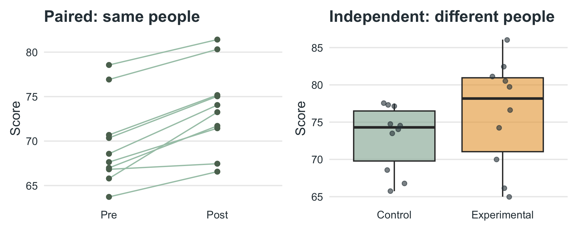
Last time, we compared two related means: the same participants measured twice (e.g., stress before vs. after a mindfulness program).

Now, we’ll compare two unrelated means: different participants in each group.

Paired t-test	Independent t-test
Same people	Different people
Within-subjects	Between-subjects
Reduces error (individual differences)	Must estimate error separately

From Paired to Independent Samples

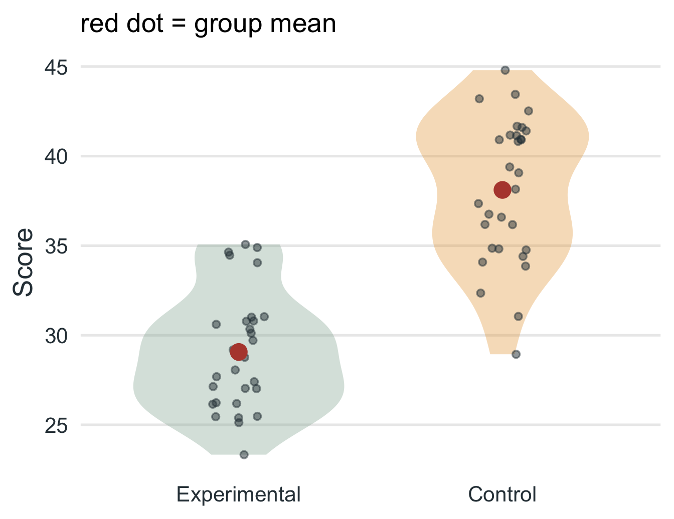
Visual comparison

Sampling Theory (Recap)

Comparing two unrelated groups

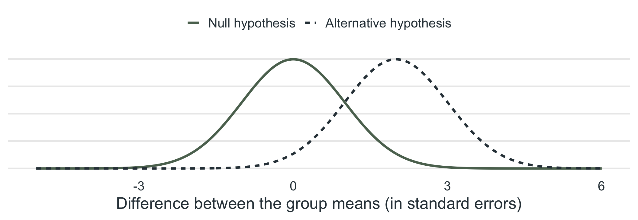
Sampling theory lets us test two unrelated groups.
Under \(H_0\) the difference between group means is centered on 0. Under \(H_A\) it is centered somewhere else.

Sampling Theory (Recap)

A difference near 0 looks like the null

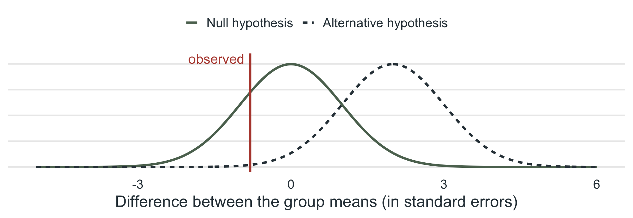
An observed difference like this is easy to produce when \(H_0\) is true.

Sampling Theory (Recap)

A difference beyond the critical value does not

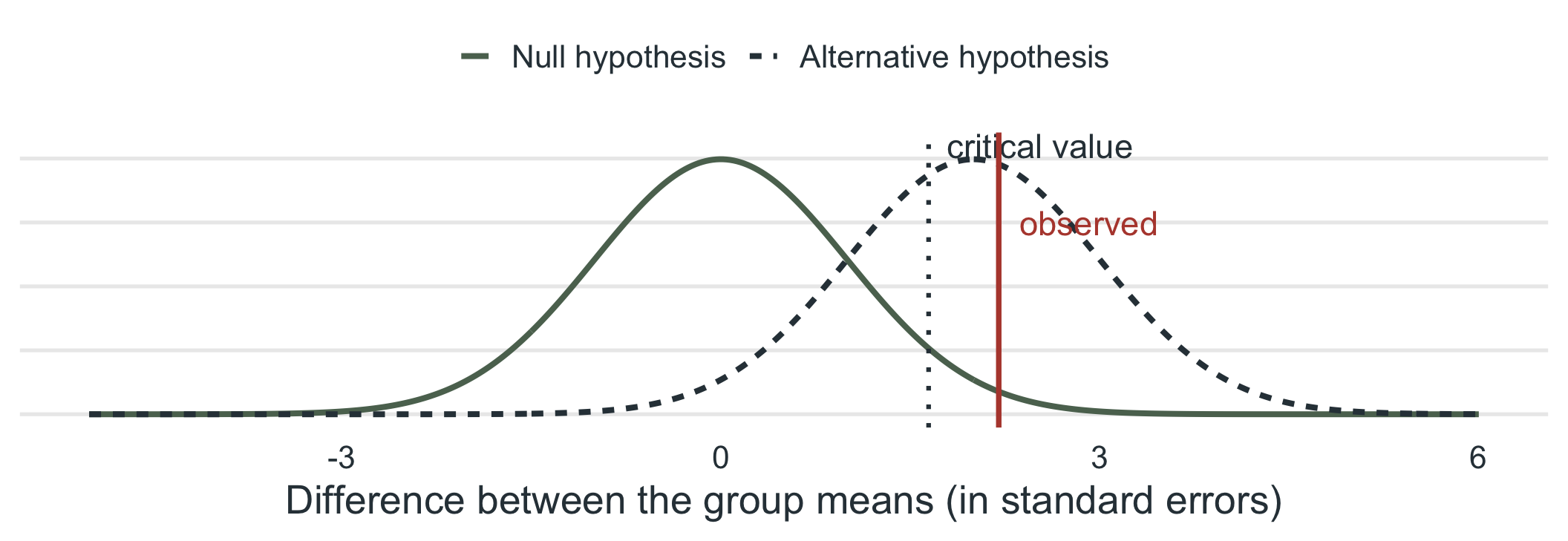
Beyond the critical value, the observed difference would be very unusual under \(H_0\), so we reject it.

Inferential Statistics

Applied to independent groups

Our goal is still to test whether a difference is likely due to chance.
With independent samples, chance variation now includes differences between individuals in both groups.

Group Variance

Within and between

To compare the means we need to know:

Between-group variance: how much the answers from the experimental group differ from the control group.
Within-group variance: how much scores differ from one another inside each group, around that group’s own mean.

Signal and Noise

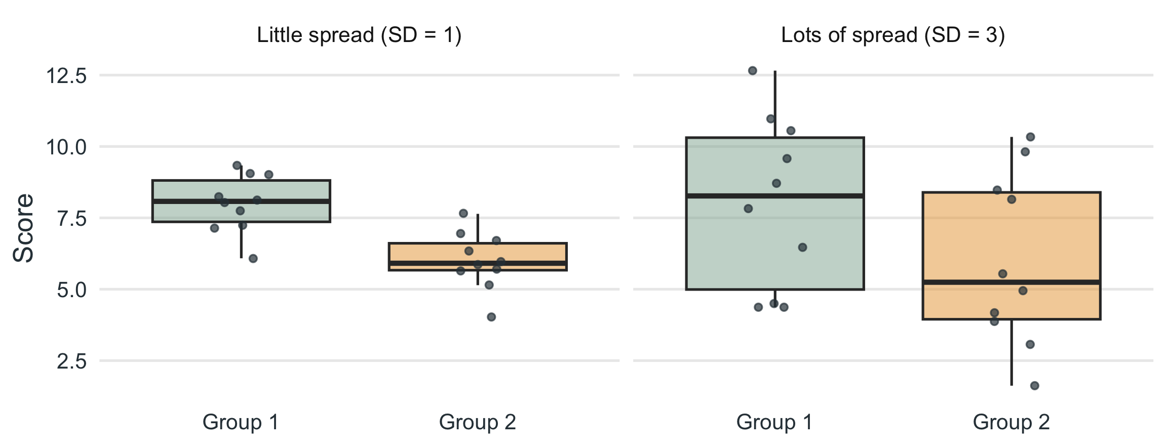
Same difference, different spread

Signal and Noise

t is signal divided by noise

\[t = \frac{\text{signal}}{\text{noise}} = \frac{\bar{x}_1 - \bar{x}_2}{SE}\]

In the previous slide, both panels have the same mean difference (\(8 - 6 = 2\)), so the same signal.
Little spread: \(t = 4.47\). Lots of spread: \(t = 1.49\). More noise means a smaller \(t\), so a difference is harder to trust.

Introduction to Independent-Samples t-Test

What is an independent-samples t-test?

Independent-Samples t-Test: A statistical method for comparing the means of two unrelated groups, such as different people randomly assigned to two conditions.

Independent-Samples t-Test Overview

Used when we compare two different groups on a continuous outcome.

local_cafe

Coffee vs. decaf

Happiness scores

headphones

Music vs. silence

Study performance

smartphone

Phone vs. no phone

Sleep quality before bed

Goal: is the mean difference between groups larger than what we’d expect by chance?

Independent-Samples t-Test

Example

The experimental group drinks caffeinated coffee. The control group drinks decaf. I ask both groups to complete a survey to measure their happiness on a scale of 1 to 10.

The experimental group has a mean happiness score of 8.
The control group has a mean happiness score of 6.

Is the group that drank coffee significantly happier than the control group?

A New Sampling Distribution

The difference between two sample means

In the one-sample test we asked how far a sample mean falls from \(\mu\).
Now there are two sample means, so the thing that bounces around from study to study is their difference, \(\bar{x}_1 - \bar{x}_2\).
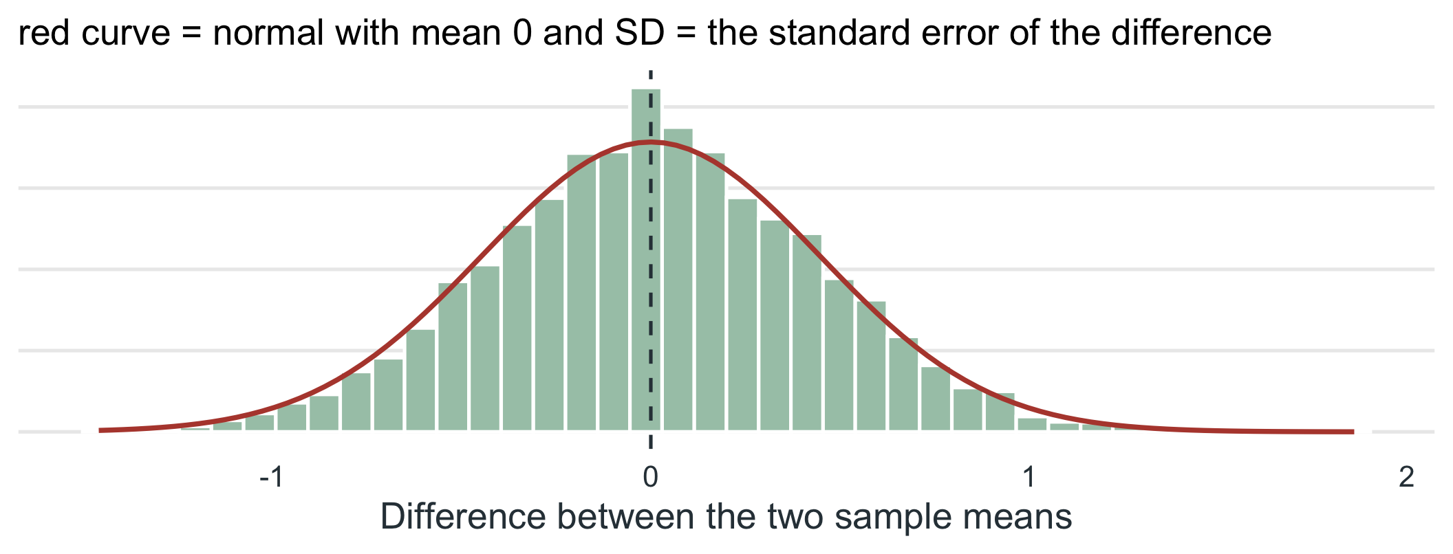
If \(H_0\) is true (both groups come from populations with the same mean), those differences pile up around 0. The test asks how far from 0 ours landed, in standard-error units.

Let’s Watch It Happen

Simulating 5000 studies

sampling_difference.R

set.seed(seed = 11)
sigma <- 1      # both populations have the same SD
n     <- 10     # people per group

# Run the "study" 5000 times with H0 true (same mean, 7, in both groups)
diffs <- replicate(n = 5000, expr = {
  group_1 <- rnorm(n = n, mean = 7, sd = sigma)
  group_2 <- rnorm(n = n, mean = 7, sd = sigma)
  mean(x = group_1) - mean(x = group_2)
})

c(simulated_sd = sd(x = diffs),
  formula = sigma * sqrt(x = 1 / n + 1 / n))

simulated_sd      formula 
   0.4321172    0.4472136

The spread of the simulated differences is the standard error of the difference, and the formula \(\sigma\sqrt{\frac{1}{n_1} + \frac{1}{n_2}}\) predicts it.

A New Sampling Distribution

What the 5000 differences look like

Why the Standard Errors Add

From one mean to a difference of two

\[SE_{\bar{x}} = \frac{\sigma}{\sqrt{n}} \qquad\Longrightarrow\qquad SE_{\bar{x}_1 - \bar{x}_2} = \sqrt{\frac{\sigma^2}{n_1} + \frac{\sigma^2}{n_2}} = \sigma\sqrt{\frac{1}{n_1} + \frac{1}{n_2}}\]

Each sample mean has its own wobble, \(\sigma^2/n_j\) (the squared standard error).
A difference inherits the wobble of both means, and variances add (even when you subtract), so the two squared standard errors add. Then we take the square root.
Two noisy means make a noisier difference than either one alone. That is why this denominator is bigger than the one-sample \(\sigma/\sqrt{n}\).

Formulas

Theoretical and computational

Inferential statistics have both theoretical and computational formulas:

Theoretical

The formula if we actually knew the population parameters (\(\sigma\)).

Computational

The formula for estimating the test statistic based solely on sample data.

Theoretical Formula

If we knew the population standard deviation

\[z = \frac{\color{#B5483B}{\bar{x}_1} - \color{#5C715E}{\bar{x}_2}}{\color{#2F3E46}{\sigma\sqrt{\frac{1}{n_1} + \frac{1}{n_2}}}}\]

The numerator is really \((\bar{x}_1 - \bar{x}_2) - (\mu_1 - \mu_2)\). Under \(H_0\) the second part is \(0\), so it drops out.
Sample mean, group 1
Sample mean, group 2
Standard error of the difference, using the population \(\sigma\) (assumed equal in both groups)

Computational Formula

Estimating from the samples (pooled t-test)

\[t = \frac{\bar{x}_1 - \bar{x}_2}{\sqrt{\color{#5C715E}{s_p^2}\left(\frac{1}{n_1} + \frac{1}{n_2}\right)}} \qquad s_p^2 = \frac{(n_1 - 1)s_1^2 + (n_2 - 1)s_2^2}{n_1 + n_2 - 2}\]

\(s_p^2\) = pooled variance, a weighted average of the two group variances.
\(df = n_1 + n_2 - 2\)

Computational Formula

When the variances are not equal (Welch’s t-test)

\[t = \frac{\bar{x}_1 - \bar{x}_2}{\sqrt{\frac{s_1^2}{n_1} + \frac{s_2^2}{n_2}}}\]

No pooling: each group’s variance keeps its own weight, and df is adjusted (it is usually not a whole number). Each \(s_j^2 = \dfrac{\sum (x_{ij} - \bar{x}_j)^2}{n_j - 1}\) is that group’s own variance: squared distances from its own mean, divided by \(n_j - 1\).
This is what t.test() does by default in R. Adding var.equal = TRUE gives the pooled version above.

Pooled or Welch: Same Idea

Both add the two squared standard errors

\[\text{Welch: } \sqrt{\frac{s_1^2}{n_1} + \frac{s_2^2}{n_2}} \qquad\qquad \text{Pooled: } \sqrt{\frac{s_p^2}{n_1} + \frac{s_p^2}{n_2}}, \quad s_p^2 = \frac{(n_1 - 1)s_1^2 + (n_2 - 1)s_2^2}{n_1 + n_2 - 2}\]

Welch lets each group keep its own variance. Pooling uses one shared \(s_p^2\), a weighted average (bigger groups count more).
With equal \(n\) and similar variances the two agree (coffee: identical \(t\)).
When variances differ a lot, \(s_p^2\) stops describing either group. Next: what goes wrong.

Where df Comes From

Two means estimated, two degrees lost

The pooled \(s_p^2\) uses two sample means (one per group) to measure spread.
Each estimated mean costs one degree of freedom: \((n_1 - 1) + (n_2 - 1) = n_1 + n_2 - 2\).
Coffee: \(10 + 10 - 2 = 18\). Welch adjusts df to account for unequal variances, so it is usually not a whole number.

Coffee Example

Manual

Pooled variance and standard error

\(s_p^2 = \dfrac{(10-1)(1)^2 + (10-1)(1)^2}{10 + 10 - 2} = 1.00\) and \(SE = \sqrt{1.00\left(\frac{1}{10} + \frac{1}{10}\right)} = 0.45\)

Compute t

\(t = \dfrac{8 - 6}{0.45} = 4.47\)

The denominator is \(SE = \sqrt{s_p^2\left(\frac{1}{n_1} + \frac{1}{n_2}\right)}\), the standard error of the difference between the two means.

Decide

\(df = 10 + 10 - 2 = 18\). At \(\alpha = .05\) (two-tailed), \(t_{critical} = \pm 2.101\). Since \(4.47 > 2.101\), we reject \(H_0\).

Coffee Example

Data overview

mdiff	t	df	p	Experimental	Control	CI[ll,uu]
2.00	4.47	18	<.001	8.00	6.00	[1.06, 2.94]

mdiff is the experimental mean minus the control mean (\(8 - 6 = 2\)). The factor levels set the order, so put the group you want first to get a positive difference.

Reading the `t.test()` Output

Every piece comes from the formula

coffee_t_test.R

t.test(formula = happy ~ grp, data = coffee)   # Welch by default


    Welch Two Sample t-test

data:  happy by grp
t = 4.4721, df = 18, p-value = 0.0002946
alternative hypothesis: true difference in means between group Experimental and group Control is not equal to 0
95 percent confidence interval:
 1.060439 2.939561
sample estimates:
mean in group Experimental      mean in group Control 
                         8                          6

Reading the `t.test()` Output

Where each number comes from

t \(= \dfrac{\text{mean difference}}{SE} = \dfrac{8 - 6}{0.45} = 4.47\). The two means are listed at the bottom, the standard error is never printed.
df is computed from the two variances (Welch). Here it equals \(n_1 + n_2 - 2 = 18\) because the groups match in size and spread. p-value is the area beyond \(\pm t\) in both tails of that \(t\) distribution.
95% CI is the mean difference \(\pm\ t_{critical} \times SE\), an interval for \(\mu_1 - \mu_2\).

Independent-Samples t-Test

Assumptions

Assumptions

DV is continuous (interval or ratio scale).
Observations are independent, and the data are randomly sampled. Each person appears in only one group.
Normality: each group’s distribution is approximately normal (or the groups are large enough for the CLT).
Equal variances (homogeneity of variance): the two groups have similar spread. Only the pooled test needs this.

Why Equal Variances?

The pooled test uses one shared variance

Pooling says: “both groups are estimating the same \(\sigma^2\), so combine them into one \(s_p^2\).”
That is only a fair summary when the groups really do have similar spread.
Say a small group is very noisy (\(n = 10\), \(s = 4\)) and a large group is steady (\(n = 40\), \(s = 1\)):

\[SE_{pooled} = 0.69 \qquad SE_{Welch} = \sqrt{\tfrac{4^2}{10} + \tfrac{1^2}{40}} = 1.27\]

The pooled version leans on the big, quiet group and understates the noise. A standard error that is too small makes \(t\) too big.

What Goes Wrong

Simulating false alarms

false_alarms.R

set.seed(seed = 348)

# Two groups with the SAME true mean (H0 is true). How often is p < .05?
one_study <- function(n1, sd1, n2, sd2) {
  x <- rnorm(n = n1, mean = 0, sd = sd1)
  y <- rnorm(n = n2, mean = 0, sd = sd2)
  c(pooled = t.test(x = x, y = y, var.equal = TRUE)$p.value,
    welch  = t.test(x = x, y = y, var.equal = FALSE)$p.value)
}

unequal <- replicate(n = 4000, expr = one_study(n1 = 10, sd1 = 4, n2 = 40, sd2 = 1))
equal   <- replicate(n = 4000, expr = one_study(n1 = 25, sd1 = 2, n2 = 25, sd2 = 2))

rbind(unequal_groups = rowMeans(x = unequal < .05),
      equal_groups   = rowMeans(x = equal < .05))

                pooled   welch
unequal_groups 0.30275 0.05275
equal_groups   0.05050 0.05025

What Goes Wrong

The false-alarm rate

We want about .05. With unequal spread and unequal \(n\), the pooled test cries wolf 30% of the time. Welch stays near 5%.
That is why we check: the pooled test is only trustworthy when the spreads are similar.

Checking Equal Variances

Look first, then test

compare_spread.R

aggregate(x = concentration ~ group, data = choco, FUN = sd)

         group concentration
1    chocolate      2.612729
2 no_chocolate      1.893840

Look: are the group SDs in the same ballpark? A rough rule is that the largest SD is no more than about twice the smallest.
Test: Levene’s Test asks the same question formally. \(H_0\): the group variances are equal.

Levene’s Test in R

One row of results, not two

levene_intro.R

library(car)
leveneTest(y = score ~ group, data = noisy)

Levene's Test for Homogeneity of Variance (center = median)
      Df F value    Pr(>F)    
group  1  18.262 9.075e-05 ***
      48                      
---
Signif. codes:  0 '***' 0.001 '**' 0.01 '*' 0.05 '.' 0.1 ' ' 1

R prints one row of results. There are no “top row / bottom row” versions to choose from. Read the Pr(>F) column: that is the \(p\)-value.
\(p < .05\): the variances differ, so do not trust the pooled test. \(p > .05\): no evidence they differ.

What R Does Instead of Two Rows

Choosing with `var.equal`

SPSS prints a “pooled” row and a “Welch” row. In R you choose with one argument:
- var.equal = FALSE (the default): Welch, no equal-variance assumption
- var.equal = TRUE: pooled, needs equal variances
Traditional route: run Levene’s Test, then pick (pooled if \(p > .05\), Welch if \(p < .05\)).
Many statisticians now always use Welch: nearly identical when variances are equal, protective when they are not.
Here, we check Levene’s Test to see whether pooling was safe, then run Welch anyway.

Looking Ahead: Sphericity

The same idea in repeated measures

The same idea comes back

Here the assumption is equal variances across groups. In a repeated-measures design with three or more conditions, the matching assumption is sphericity: the difference scores between every pair of conditions have similar variance.

The paired \(t\)-test never needed it, because two conditions give only one set of differences.

Let’s Apply It

Three independent designs

We’ll test three common between-subjects designs:

Chocolate and Concentration

Experimental vs. control

headphones

Music and Studying

Environmental manipulation

smartphone

Phone Use and Sleep

Behavioral difference

Does chocolate improve concentration?

Design

50 undergraduate students from XYZ University were randomly assigned to one of two groups. One group received a small piece of chocolate (70% dark cocoa) to consume before completing a 10-minute concentration task. The other group received no chocolate. The task measured sustained attention and was scored on a 0-20 scale.

IV: chocolate (yes vs. no)
DV: concentration task score
Design: between-subjects, randomized

Does chocolate improve concentration?

Hypotheses

Null hypothesis \(H_0\)

Concentration is the same with and without chocolate.

\(\mu_\text{chocolate} = \mu_\text{no chocolate}\)

Alternative hypothesis \(H_A\)

Concentration differs between the groups.

\(\mu_\text{chocolate} \neq \mu_\text{no chocolate}\)

Does chocolate improve concentration?

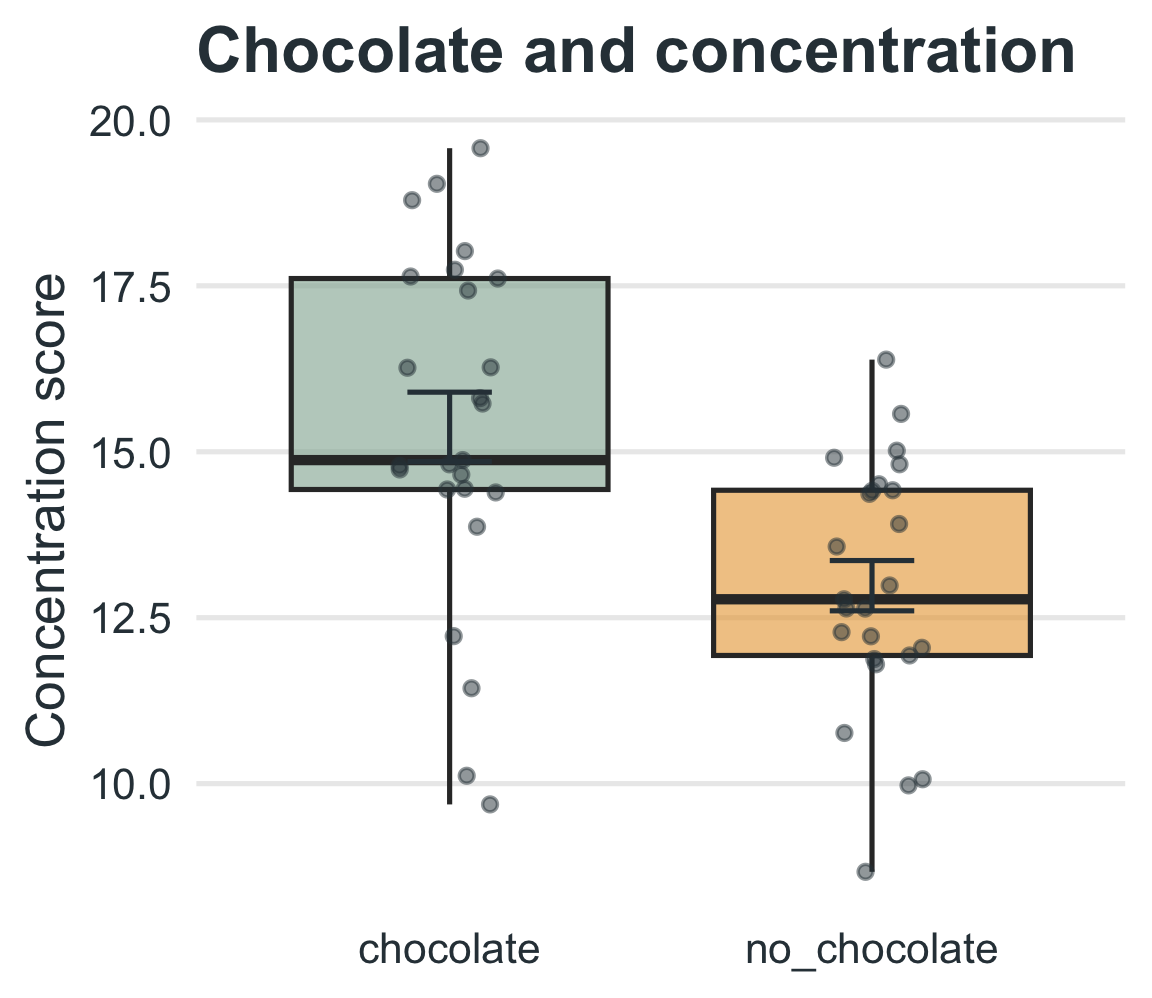
Data and results

Difference	t	df	p	CI[ll,uu]	d
2.39	3.71	43.76	<.001	[1.09, 3.69]	1.05

Chocolate: \(M = 15.38\), \(SD = 2.61\). No chocolate: \(M = 12.98\), \(SD = 1.89\).

Does chocolate improve concentration?

Check the assumption

levene.R

library(car)

# Equal variances? (H0: the variances are equal)
leveneTest(y = concentration ~ group, data = choco)

Levene's Test for Homogeneity of Variance (center = median)
      Df F value Pr(>F)
group  1  1.4945 0.2275
      48

Levene’s \(p > .05\), so equal variances are reasonable and pooling would have been fine. We run Welch anyway: it is safe either way.

Does chocolate improve concentration?

Run the test

chocolate.R

# Welch (R's default): no equal-variance assumption
t.test(formula = concentration ~ group, data = choco)


    Welch Two Sample t-test

data:  concentration by group
t = 3.7076, df = 43.764, p-value = 0.0005855
alternative hypothesis: true difference in means between group chocolate and group no_chocolate is not equal to 0
95 percent confidence interval:
 1.091949 3.693714
sample estimates:
   mean in group chocolate mean in group no_chocolate 
                  15.37507                   12.98224

Does chocolate improve concentration?

Decision, effect size, and report

Decide

\(t(43.76) = 3.71\), \(p\) < .001. Since \(p < .05\), we reject \(H_0\).

Effect size

\(d = \dfrac{\bar{x}_1 - \bar{x}_2}{s_p} = \dfrac{2.39}{2.28} = 1.05\) (a large effect), where \(s_p = \sqrt{s_p^2}\) is the square root of the pooled variance

An independent-samples t-test showed that students who ate chocolate (M = 15.38, SD = 2.61) scored significantly higher on the concentration task than students who did not (M = 12.98, SD = 1.89), t(43.76) = 3.71, p < .001, 95% CI [1.09, 3.69], d = 1.05.

Does instrumental music improve studying?

Design

Design Summary
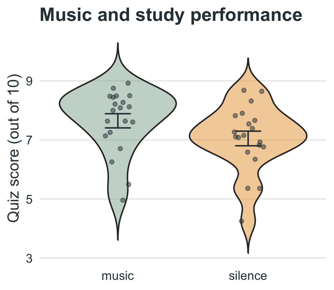
40 students participated in a study examining how background music affects studying. Participants were randomly assigned to study a short academic text under one of two conditions: instrumental music or silence. After 15 minutes of study time, they completed a 10-item multiple-choice quiz.

IV: study condition (instrumental music vs. silence)
DV: quiz performance (number of correct answers out of 10)
Design: between-subjects, randomized

Does instrumental music improve studying?

Hypotheses

Null hypothesis \(H_0\)

Quiz performance is the same with music and in silence.

\(\mu_\text{music} = \mu_\text{silence}\)

Alternative hypothesis \(H_A\)

Quiz performance differs between the conditions.

\(\mu_\text{music} \neq \mu_\text{silence}\)

Does instrumental music improve studying?

Data and results

Difference	t	df	p	CI[ll,uu]	d
0.60	1.73	37.96	0.091	[-0.10, 1.30]	0.55

Music: \(M = 7.65\), \(SD = 1.08\). Silence: \(M = 7.05\), \(SD = 1.11\).

Does instrumental music improve studying?

Run the test

music.R

# Welch (R's default)
t.test(formula = quiz_score ~ group, data = music)


    Welch Two Sample t-test

data:  quiz_score by group
t = 1.7335, df = 37.964, p-value = 0.09112
alternative hypothesis: true difference in means between group music and group silence is not equal to 0
95 percent confidence interval:
 -0.1005039  1.2980783
sample estimates:
  mean in group music mean in group silence 
             7.647986              7.049199

Does instrumental music improve studying?

Decision, effect size, and report

Decide

\(t(37.96) = 1.73\), \(p\) = .091. Since \(p > .05\), we fail to reject \(H_0\).

Effect size

\(d = \dfrac{0.60}{1.09} = 0.55\) (a medium effect)

An independent-samples t-test showed that students who studied with music (M = 7.65, SD = 1.08) did not differ significantly on the quiz from students who studied in silence (M = 7.05, SD = 1.11), t(37.96) = 1.73, p = .091, 95% CI [-0.10, 1.30], d = 0.55.

Does instrumental music improve studying?

Reading a non-significant result

A medium effect that is not significant is a hint that the study may have been too small to detect it. (If we had predicted a direction before collecting data, the one-tailed \(p\) would be about 0.046. But the direction has to be chosen before you see the result.)

Does bedtime phone use affect sleep?

Design

Design Summary
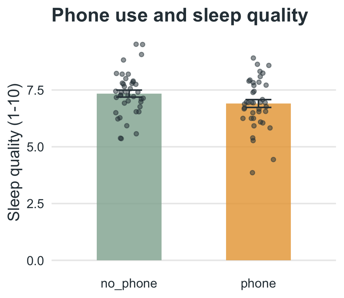
80 students were randomly assigned to avoid phone use for 30 minutes before bed or to use their phones as normal. The next morning, all students rated their sleep quality on a 1-10 scale.

IV: phone use before bed (yes vs. no)
DV: sleep quality rating (1 = poor, 10 = excellent)
Design: between-subjects, randomized

Does bedtime phone use affect sleep?

Hypotheses

Null hypothesis \(H_0\)

Sleep quality is the same with and without bedtime phone use.

\(\mu_\text{no phone} = \mu_\text{phone}\)

Alternative hypothesis \(H_A\)

Sleep quality differs between the conditions.

\(\mu_\text{no phone} \neq \mu_\text{phone}\)

Does bedtime phone use affect sleep?

Data and results

Difference	t	df	p	CI[ll,uu]	d
0.44	1.89	77.01	0.063	[-0.02, 0.90]	0.42

No phone: \(M = 7.34\), \(SD = 0.97\). Phone: \(M = 6.90\), \(SD = 1.09\).

Does bedtime phone use affect sleep?

Run the test

sleep.R

# Welch (R's default)
t.test(formula = sleep_quality ~ group, data = sleep)


    Welch Two Sample t-test

data:  sleep_quality by group
t = 1.89, df = 77.011, p-value = 0.06253
alternative hypothesis: true difference in means between group no_phone and group phone is not equal to 0
95 percent confidence interval:
 -0.02339518  0.89648805
sample estimates:
mean in group no_phone    mean in group phone 
              7.341146               6.904599

Does bedtime phone use affect sleep?

Decision, effect size, and report

Decide

\(t(77.01) = 1.89\), \(p\) = .063. Since \(p > .05\), we fail to reject \(H_0\). The result is close, but not significant.

Effect size

\(d = \dfrac{0.44}{1.03} = 0.42\) (a small-to-medium effect)

An independent-samples t-test showed that students who avoided their phones before bed (M = 7.34, SD = 0.97) did not differ significantly in sleep quality from students who used their phones (M = 6.90, SD = 1.09), t(77.01) = 1.89, p = .063, 95% CI [-0.02, 0.90], d = 0.42.

Practice

Caffeine and alertness

Does caffeine increase alertness? 40 participants were randomly assigned to caffeine or a placebo (ex_3: Group, Alertness; 20 per group). Alertness was scored on a 0-100 scale.

Your tasks

State \(H_0\) and \(H_A\).
Check the equal-variance assumption (Levene’s Test).
Run the independent-samples t-test, compute \(d\), and write an APA sentence.

Practice

Caffeine and alertness: data and answer

practice_3.R

set.seed(103)
ex_3 <- tibble(
  Group = factor(rep(c("Caffeine", "Placebo"), each = 20),
                 levels = c("Caffeine", "Placebo")),
  Alertness = c(rnorm(20, mean = 75, sd = 8), rnorm(20, mean = 68, sd = 8))
)

Answer

\(H_0: \mu_\text{caffeine} = \mu_\text{placebo}\); \(H_A: \mu_\text{caffeine} \neq \mu_\text{placebo}\). Caffeine \(M = 74.31\) vs. placebo \(M = 68.23\): t(37.93) = 2.52, p = .016, 95% CI [1.19, 10.98], \(d = 0.80\).

Practice

Online vs. in-person exams

Do exam scores differ between online and in-person sections? 25 students in each format took the same exam (ex_4: Format, Exam_Score).

Your tasks

State \(H_0\) and \(H_A\).
Check the equal-variance assumption (Levene’s Test).
Run the independent-samples t-test, compute \(d\), and decide.

Practice

Online vs. in-person exams: data and answer

practice_4.R

set.seed(104)
ex_4 <- tibble(
  Format = factor(rep(c("Online", "InPerson"), each = 25),
                  levels = c("Online", "InPerson")),
  Exam_Score = c(rnorm(25, mean = 82, sd = 5), rnorm(25, mean = 79, sd = 6))
)

Answer

\(H_0: \mu_\text{online} = \mu_\text{in-person}\); \(H_A: \mu_\text{online} \neq \mu_\text{in-person}\). Online \(M = 81.99\) vs. in-person \(M = 78.52\): t(46.29) = 2.70, p = .010, \(d = 0.76\). Compare \(p\) to \(\alpha = .05\) and interpret both the decision and the effect size.

Terms to Know

The vocabulary for this test

Standard error of the difference: How much the difference between two sample means bounces around from study to study. It is the denominator of \(t\).

Pooled variance \(s_p^2\): A weighted average of the two group variances, used when the groups are assumed to share one population variance.

Welch’s t-test: An independent-samples \(t\)-test that lets each group keep its own variance. It is the default in t.test().

Levene’s test: A test of \(H_0\) that the group variances are equal.

Summary: Independent-Samples t-Test

Compares two independent groups.
Tests whether the difference in means is significant.
Welch’s t-test (R’s default) does not assume equal variances. The pooled version needs them.
Check assumptions: independence, normality, equal variance (look at the SDs, then Levene’s Test, or just use Welch).
Report the test, the means and SDs, the confidence interval, and an effect size (\(d\)).

Independent-Samples T-Test

From Paired to Independent Samples

From Paired to Independent Samples

Visual comparison

Sampling Theory (Recap)

Comparing two unrelated groups

Sampling Theory (Recap)

A difference near 0 looks like the null

Sampling Theory (Recap)

A difference beyond the critical value does not

Inferential Statistics

Applied to independent groups

Group Variance

Within and between

Signal and Noise

Same difference, different spread

Signal and Noise

t is signal divided by noise

Introduction to Independent-Samples t-Test

What is an independent-samples t-test?

Independent-Samples t-Test Overview

Coffee vs. decaf

Music vs. silence

Phone vs. no phone

Independent-Samples t-Test

Example

A New Sampling Distribution

The difference between two sample means

Let’s Watch It Happen

Simulating 5000 studies

A New Sampling Distribution

What the 5000 differences look like

Why the Standard Errors Add

From one mean to a difference of two

Formulas

Theoretical and computational

Theoretical Formula

If we knew the population standard deviation

Computational Formula

Estimating from the samples (pooled t-test)

Computational Formula

When the variances are not equal (Welch’s t-test)

Pooled or Welch: Same Idea

Both add the two squared standard errors

Where df Comes From

Two means estimated, two degrees lost

Coffee Example

Manual

Coffee Example

Data overview

Reading the t.test() Output

Every piece comes from the formula

Reading the t.test() Output

Where each number comes from

Independent-Samples t-Test

Assumptions

Why Equal Variances?

The pooled test uses one shared variance

What Goes Wrong

Simulating false alarms

What Goes Wrong

The false-alarm rate

Checking Equal Variances

Look first, then test

Levene’s Test in R

One row of results, not two

What R Does Instead of Two Rows

Choosing with var.equal

Looking Ahead: Sphericity

The same idea in repeated measures

Let’s Apply It

Three independent designs

Chocolate and Concentration

Music and Studying

Phone Use and Sleep

Does chocolate improve concentration?

Design

Does chocolate improve concentration?

Hypotheses

Does chocolate improve concentration?

Reading the `t.test()` Output

Reading the `t.test()` Output

Choosing with `var.equal`