Linear Regression

Lecture 11

Dave Brocker

Farmingdale State College

Types of Analysis

Univariate: One variable, like the mean
Bivariate: Two variables, like correlation
Multivariate: More than 2 variables

Regression

Regression is the multivariate version of correlation.
Correlation is the bivariate version of regression.
We’re doing the same thing in regression as we do in correlation, BUT there are more than 2 variables.

Regression terminology

In regression we will choose one variable to predict.

We call this $Y$.
$Y$ is the outcome variable.
$\hat{Y}$ is the predicted variable.

Regression terminology

In regression we will choose two or more variables we have reason to believe predict y.

We call these $A$, $B$, etc.
$A$ is the predictor variable.

Regression terminology

When we predict Y with X, we say;

We regress y on the x.

Regression Equation

Step-by-Step

\[ \large{\color{red}{Y_i} = \color{green}{\beta_0} + \color{blue}{\beta_1(A)}+\color{orange}{e_i}} \]

1. The predicted value of y for a particular participant (i)

2. Intercept: Value of Y when all other predictors are 0

3. Weight

4. The Value of a particular participant on the measure of $A$

5. Error. Random, and therefore cannot be predicted

Regression Equation

A Few Ways to Write the Same Thing!

\[ \large{\color{red}{Y_i} = \color{green}{\beta_0} + \color{blue}{\beta_1(A)}} \]

\[\hat{Y} = \beta_0 + \beta_1(A)\]

\[Y = ax + b\]

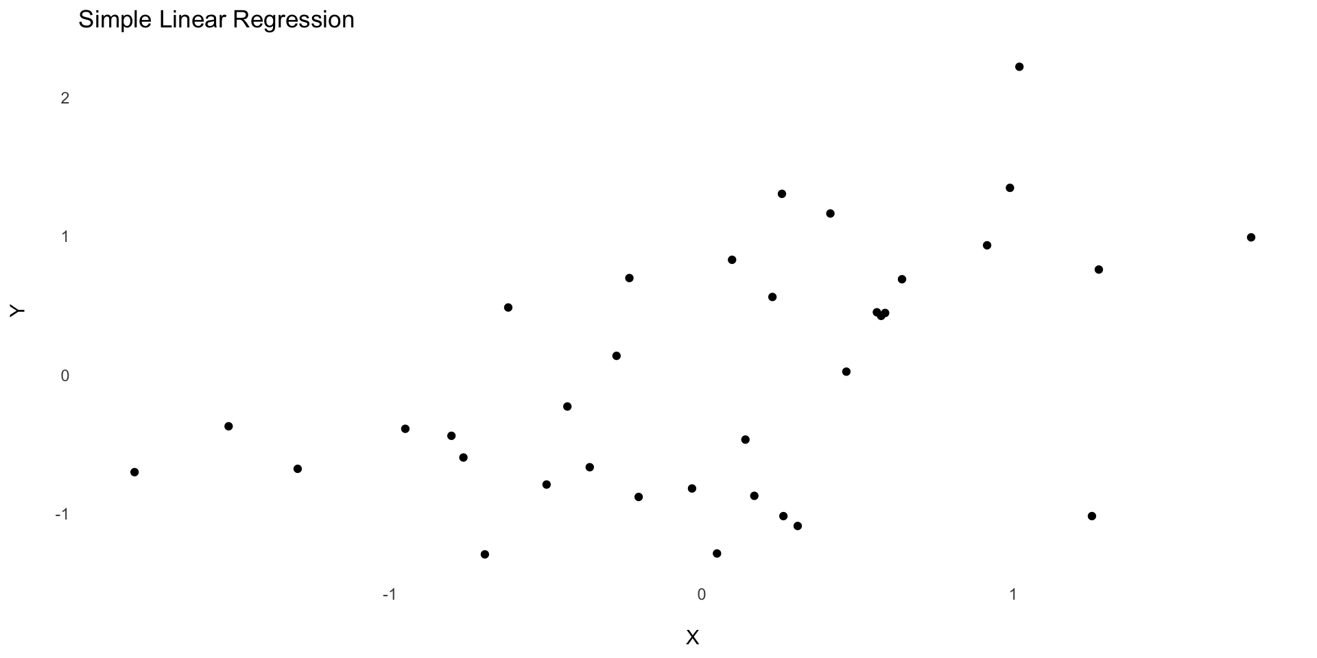
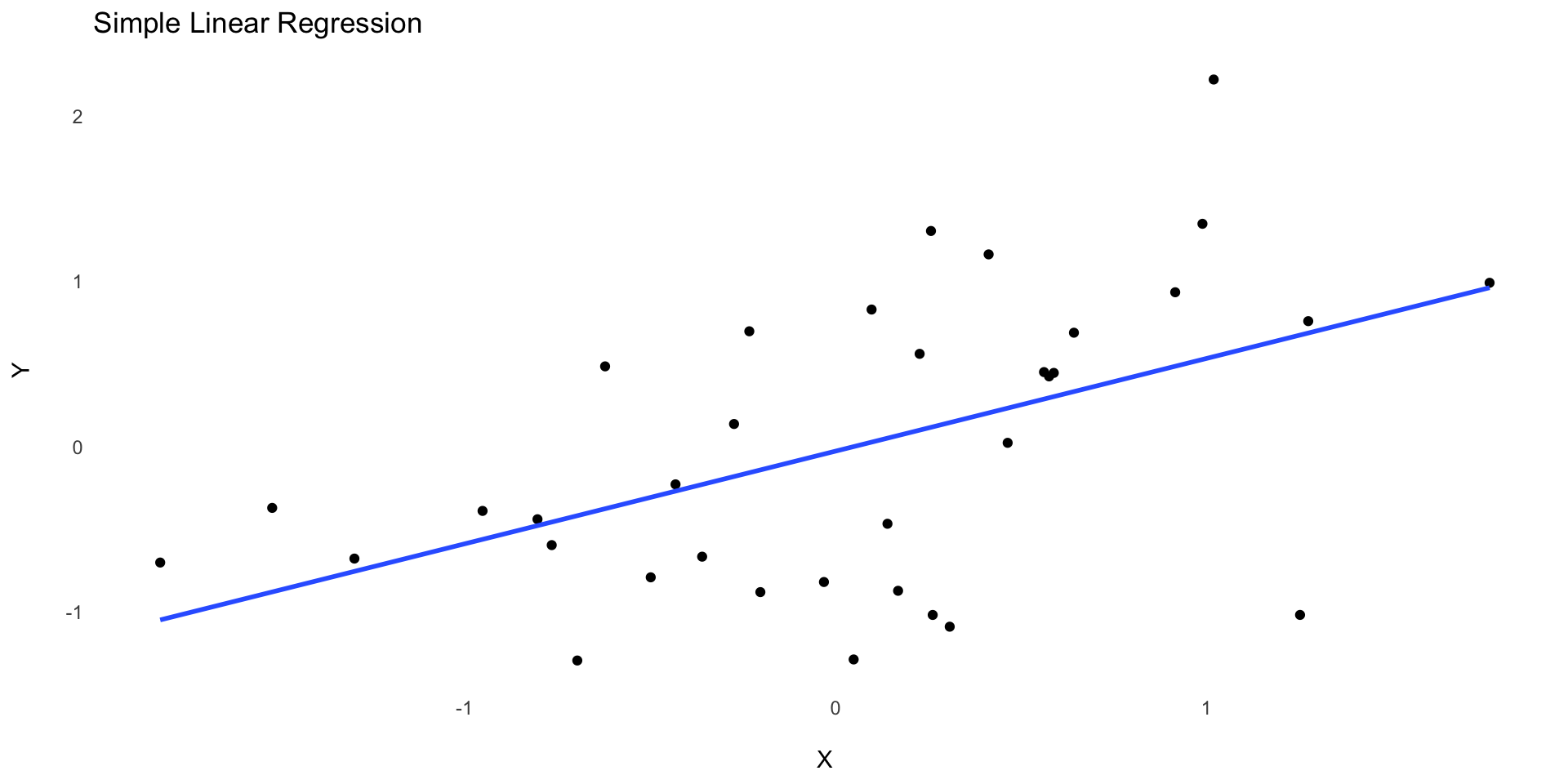
Linear Regression

Regression:

Equation Component Meanings

$Y$ = theoretical prediction of y
$\hat{Y}$= the actual y value for a participant
$\beta_0$ = the intercept: the average y value
$A$ = the A value for a participant
$\beta_1$ = a weighted value that is multiplied by A and added to $\beta_0$ to estimate y.

Regression Equation:

More than one X

$\large{\hat{Y}_i = \beta_0 + \beta_1(A) + \beta_2(B)}...$

Regression:

Equation Component Meanings

$Y$ = theoretical prediction of y
$\hat{Y}$= the actual y value for a participant
$\beta_0$ = the intercept: the average y value
$A$ = the $A$ value for a participant
$\beta_1$ = a weighted value that is multiplied by x and added to $\beta_0$ to estimate y.
$B$ = the $B$ value for a participant
$\beta_2$ = a weighted value that is multiplied by $B$

Regression Equation:

More than one X

$\hat{Y}_i = \beta_0 + \beta_1(A) + \beta_2(B)$

Interpreting Coefficients

Regression Model Table

Two Predictor Variables

Characteristic	Beta	95% CI	p-value
x1	0.23	-0.28, 0.74	0.4
x2	0.05	-0.42, 0.52	0.8
Abbreviation: CI = Confidence Interval

Interpreting coefficients

Beta coefficient
t-value
p-value

Interpreting coefficients

Beta coefficient
t-value
p-value: is this a significant predictor of y?

Interpreting coefficients

Beta coefficient: which predictor of y has the more predictive power?
t-value
p-value

$R^2$: Coefficient of Determination

How much can we account for?

$R^2$ is the correlation coefficient (r) squared.
$R^2$ is always positive
In correlation, the amount of y accounted for by x

$R^2$: Coefficient of Determination

How much can we account for?

In Regression, $R^2$ refers to the amount of y accounted for by all of the x's.
How much of y did we account for?
Did we account for a significant amount of the variance in y?

$R^2$: Coefficient of Determination

How much can we account for?

Interpreting R Squared

R Squared
Adjusted R Squared
F-value
p-value: is this a significant predictor of y?

Interpreting R Squared

R Squared: The percentage of y accounted for by the predictors
Adjusted R Squared
F-value
p-value

Interpreting R Squared

R Squared
Adjusted R Squared: The percentage of y accounted for by the predictors, controlling for using too many predictors
F-value
p-value

Linear Regression Example

Linear Regression

Example

Professor Brocker wants to be able to predict social media use. The Social Media Use Scale measures different motivations and reasons for using Social Media platforms.

What are some predictors of social media use?

Sense of belonging
Age

Regression Equation

\[\large{Y_i = \beta_0 + \beta_1A + \beta_2B~ + e_i}\]

Regression Equation

Theoretical

\[\large{\color{red}{Y_i} = \color{green}{\beta_0} + \color{orange}{\beta_1}\color{blue}{(Age)} + \color{purple}{\beta_2(SOB)}\color{pink}~ + e_i}\]

The predicted degree of social media use for a participant “i”
Intercept: Average social media use when all other predictors are 0.
Coefficient for $A$
What is the sense of belonging?
Coefficient for $B$
Age
Randomness

Regression Equation

Computational

$\hat{Y}_i = \beta_0 + \beta_1(A) + \beta_2(B)$

Linear Regression

This form of regression is called linear regression.

Example

Model Coefficients

Social Media Use Model
Characteristic	Beta	95% CI	p-value
(Intercept)	5.2	4.3, 6.1	<0.001
Age	-0.10	-0.13, -0.08	<0.001
Sense_of_Belonging	0.29	0.22, 0.36	<0.001
Abbreviation: CI = Confidence Interval

Regression Model Summary
Predicting Social Media Use for Age and Sense of Belonging
Metric	Value
Residual Standard Error	0.512
Multiple R-squared	0.87
Adjusted R-squared	0.861
F-statistic	90.681
p	1.046 × 10⁻¹²

Reporting Regression Findings

Example

First, report adjusted $R^2$ and it’s corresponding p:

Our model predicted a significant amount of variance in social media use, adjusted $R^2$ = 0.86, p* < 0.001.
Age, sense of belonging, predicted a significant amount of variance in social media use, adjusted $R^2$ = 0.86, p < 0.001.

Example

Social Media Use Model
Characteristic	Beta	95% CI	p-value
(Intercept)	5.2	4.3, 6.1	<0.001
Age	-0.10	-0.13, -0.08	<0.001
Sense_of_Belonging	0.29	0.22, 0.36	<0.001
Abbreviation: CI = Confidence Interval

Then report individual betas and their p’s:

Sense of belonging (beta = 0.29, p = 0.001) significantly predicted social media use.
Age significantly predicted likelihood of social media use (beta = -.10, p <.001)
It’s common to report betas and p’s in text as well as in a table.

Categorical Variables in Regression

Multiple Predictors

Understanding the Factors That Influence Energy Levels

What determines how energized you feel throughout the day? Is it the number of cups of coffee you drink? The amount of sleep you got the night before? Or maybe even the type of TV shows you watch before bed?

Multiple Predictors

Understanding the Factors That Influence Energy Levels

In this example, we explore how TV watching habits (duration and genre), caffeine intake, and prior sleep predict energy levels. Using a multiple regression model, we’ll examine:

Duration of TV Watching (Continuous) – Does watching more TV affect energy?
Cups of Coffee (Continuous) – Does caffeine actually help?
Prior Sleep (Continuous) – Does more sleep always mean more energy?
TV Genre (Categorical: Drama, Comedy, Documentary) – Can what you watch impact how you feel?

Categorical variables

Fit the Model

Energy Level Model
What is the best predictor?
Characteristic	Beta	95% CI	p-value
(Intercept)	3.2	1.8, 4.5	<0.001
Duration_TV	1.2	0.93, 1.4	<0.001
Cups_of_Coffee	0.62	0.43, 0.81	<0.001
Prior_Sleep	-0.37	-0.54, -0.21	<0.001
TV_Genre
Comedy	—	—
Documentary	3.2	2.6, 3.8	<0.001
Drama	1.5	0.63, 2.4	0.002
Abbreviation: CI = Confidence Interval

Horror Movies

Characteristic	Beta	95% CI	p-value
Ranking	-0.01	-0.04, 0.02	0.5
Avg. Heart Rate (BPM)	-0.04	-0.27, 0.18	0.7
Overall Difference (BPM)	1.8	1.6, 2.1	<0.001
HRV Difference	1.6	1.5, 1.6	<0.001
Highest Spike	0.18	0.17, 0.19	<0.001
Sequel
no	—	—
yes	0.00	-0.24, 0.25	>0.9
At Least One Sequel
no	—	—
yes	-0.03	-0.28, 0.22	0.8
Rotten Tomato Score	0.00	0.00, 0.01	0.8
Year	0.00	-0.01, 0.01	0.4
Abbreviation: CI = Confidence Interval

Review Questions

Multiple-Choice Questions

1. What does the slope in a simple linear regression equation represent?

A) The value of Y when X = 0

B) The predicted change in Y for a one-unit increase in X

C) The strength of the correlation between X and Y

D) The proportion of variance in Y explained by X

2. If a linear regression model has an R² value of 0.85, what does this mean?

A) 85% of the variability in X is explained by Y

B) The regression model is 85% accurate

C) 85% of the variability in Y is explained by X D) The relationship between X and Y is statistically significant

3. A researcher runs a regression model and finds the following equation:

What does the number 5 represent?

A) The slope of the regression line

B) The predicted value of Y when X = 0

C) The effect size of X on Y

D) The p-value of the regression

4. Which of the following would indicate that a multiple regression model is overfitting?

A) A high R² value on the training data but poor performance on new data

B) A non-significant p-value for the intercept

C) The presence of a negative coefficient in the model D) A low standard error for the slope

5. A regression model predicts salary based on years of experience. The p-value for the slope is 0.0003. What does this mean?

A) Years of experience does not significantly predict salary

B) Years of experience significantly predicts salary at the α = 0.05 level

C) The slope coefficient is 0.0003

D) The model is not linear

Open-Ended Questions (Show Your Work)

6. A multiple regression model is given by:

$\hat{Y} = 3 + 1.5X_1 - 0.7X_2$

where:

• $X_1$ = Number of hours spent studying

• $X_2$ = Number of hours spent watching TV

a) Predict the outcome if a student studies for 6 hours and watches TV for 2 hours.

3 + (1.56) + (.72)

13.4

b) Interpret the coefficient of .

7. A researcher runs a simple linear regression and obtains the following output:

Predictor	Coefficient	Std. Error	p-value
Intercept	4.2	.5	.001
X	1.8	.3	.0005

a) Write the regression equation.

b) Interpret the slope in context.

c) If X = 10, predict Y.

8. A study investigates the relationship between sleep (X) and energy levels (Y). The model output is: $\hat{Y} = 2 + 3X$

What is the residual for a participant who slept 5 hours and had an energy level of 18?

Linear Regression

Types of Analysis

Regression

Regression terminology

Regression terminology

Regression terminology

Regression Equation

Step-by-Step

Regression Equation

A Few Ways to Write the Same Thing!

Linear Regression

Line of Best Fit

Regression:

Equation Component Meanings

Regression Equation:

More than one X

Regression:

Equation Component Meanings

Regression Equation:

More than one X

Interpreting Coefficients

Regression Model Table

Two Predictor Variables

Interpreting coefficients

Interpreting coefficients

Interpreting coefficients

\(R^2\): Coefficient of Determination

How much can we account for?

\(R^2\): Coefficient of Determination

How much can we account for?

\(R^2\): Coefficient of Determination

How much can we account for?

Interpreting R Squared

Interpreting R Squared

Interpreting R Squared

Linear Regression Example

Linear Regression

Example

Regression Equation

Regression Equation

Theoretical

Regression Equation

Computational

Linear Regression

Example

Model Coefficients

Reporting Regression Findings

Example

Example

Categorical Variables in Regression

Multiple Predictors

Understanding the Factors That Influence Energy Levels

Multiple Predictors

Understanding the Factors That Influence Energy Levels

Categorical variables

Fit the Model

Horror Movies

Review Questions

1. What does the slope in a simple linear regression equation represent?

2. If a linear regression model has an R² value of 0.85, what does this mean?

3. A researcher runs a regression model and finds the following equation:

4. Which of the following would indicate that a multiple regression model is overfitting?

5. A regression model predicts salary based on years of experience. The p-value for the slope is 0.0003. What does this mean?

Open-Ended Questions (Show Your Work)

6. A multiple regression model is given by:

7. A researcher runs a simple linear regression and obtains the following output:

8. A study investigates the relationship between sleep (X) and energy levels (Y). The model output is: $\hat{Y} = 2 + 3X$