| Participant | Pre | Post | |
|---|---|---|---|
| 1 | P1 | 10 | 7 |
| 2 | P2 | 7 | 7 |
| 3 | P3 | 12 | 11 |
| 4 | P4 | 5 | 5 |
| 5 | P5 | 7 | 4 |
| 6 | P6 | 9 | 4 |
| 7..29 | |||
| 30 | P30 | 7 | 6 |
Paired-Samples T-Test
PSY 348: Lecture 10
Dave Brocker
Farmingdale State College
Introduction to Paired-Samples t-Test
What is a paired-samples t-test?
- Paired-Samples t-Test
- A statistical method for comparing the means of two related sets of scores, such as the same people measured twice.
Purpose of Paired-Samples t-Test
Why use it?
To determine whether there is a statistically significant difference between two related group means.
Useful in psychology for assessing change due to an intervention, therapy, or experiment.
Application of Paired-Samples t-Test
When to apply this test
trending_up
Pretest-Posttest
The same group measured before and after
people
Matched Pairs
Twins or matched participants
repeat
Repeated Measures
The same group under different conditions
Connection to the One-Sample t-Test
A paired-samples t-test is a one-sample t-test on the difference scores.
One-sample
\(t = \dfrac{\bar{x} - \mu_0}{s / \sqrt{n}}\)
Is the sample mean different from a known value?
Paired
\(t = \dfrac{\bar{D} - 0}{s_D / \sqrt{n}}\)
Is the mean difference \(\bar{D}\) different from 0?
Formula for Paired-Samples t-Test
Mathematical representation
Paired-Samples t-Test
\(\large{t = \dfrac{\color{#B5483B}{\bar{D}}}{\color{#5C715E}{s_D}/\sqrt{n}}}\)
\(\color{#B5483B}{\bar{D}}\): mean of the differences between paired observations.
\(\color{#5C715E}{s_D}\): standard deviation of the differences.
\(n\): number of pairs.
Degrees of freedom: \(df = n - 1\).
Difference Scores
Where \(\color{#B5483B}{\bar{D}}\) and \(\color{#5C715E}{s_D}\) come from
\[D_i = x_{i,\text{post}} - x_{i,\text{pre}} \qquad \color{#B5483B}{\bar{D}} = \dfrac{\sum D_i}{n} \qquad \color{#5C715E}{s_D} = \sqrt{\dfrac{\sum (D_i - \bar{D})^2}{n-1}}\]
- \(D_i\) is each person’s own change (post minus pre)
- \(\bar{D}\) is the average of those changes
- \(s_D\) is how much the changes vary from one person to the next
Theoretical Formula Explanation
Understanding each component
- Mean difference \(\bar{D}\)
- The average of the differences between paired scores.
- SD of differences \(s_D\)
- How much individual differences vary around the mean difference.
- Number of pairs \(n\)
- A larger \(n\) shrinks the standard error \(s_D/\sqrt{n}\), so smaller differences can reach significance.
Paired-Samples t-Test
Application in psychology research
A psychologist measures stress levels of a group before and after a mindfulness program. Participants first answer a stress survey, next they participate in a mindfulness exercise. After the exercise, their stress scores are measured again and compared.
Steps
- State the null and alternative hypotheses.
- Calculate the difference between post- and pre-intervention scores.
- Find the mean \(\bar{D}\) and standard deviation \(s_D\) of the differences.
- Apply the formula to calculate the t-value and check for significance.
Paired-Samples t-Test
Step 1: hypotheses
Null hypothesis \(H_0\)
There will be no difference in stress before and after the mindfulness exercise.
\(\mu_\text{post} = \mu_\text{pre}\), or equivalently \(\mu_D = 0\)
Alternative hypothesis \(H_A\)
There will be a decrease in stress after the mindfulness exercise.
\(\mu_\text{post} < \mu_\text{pre}\), or equivalently \(\mu_D < 0\)
Paired-Samples t-Test
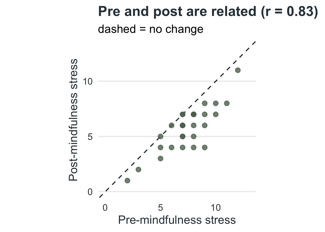
Each person has two scores
Paired-Samples t-Test
Step 2: the difference scores
| Participant | Pre | Post | D = Post - Pre | |
|---|---|---|---|---|
| 1 | P1 | 10 | 7 | -3 |
| 2 | P2 | 7 | 7 | 0 |
| 3 | P3 | 12 | 11 | -1 |
| 4 | P4 | 5 | 5 | 0 |
| 5 | P5 | 7 | 4 | -3 |
| 6 | P6 | 9 | 4 | -5 |
| 7..29 | ||||
| 30 | P30 | 7 | 6 | -1 |
\(D\) is post minus pre.
A negative \(D\) means stress went down.
From here on, the test only looks at the column of \(D\) values.
Paired-Samples t-Test
Steps 3 and 4: construct the formula (manually)
Mean and SD of the differences
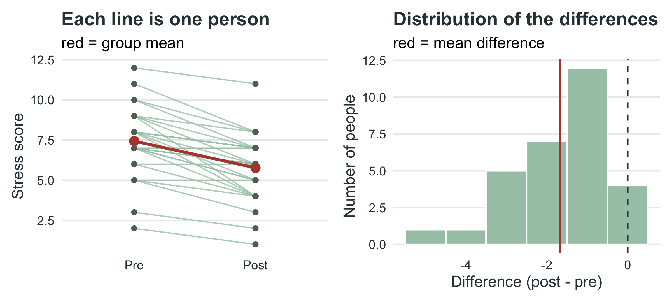
\(\bar{D} = -1.67\) and \(s_D = 1.21\) across \(n = 30\) pairs
Compute t
\(t = \dfrac{\bar{D}}{s_D/\sqrt{n}} = \dfrac{-1.67}{1.21/\sqrt{30}} = -7.53\)
Decide
At \(\alpha = .05\) (two-tailed) and \(df = 29\), \(t_{critical} = \pm 2.045\). Since \(|t| = 7.53 > 2.045\), we reject \(H_0\).
Paired-Samples t-Test
Construct the formula (computationally)
paired_t.R
    Paired t-test

data:  stress$Post and stress$Pre
t = -7.526, df = 29, p-value = 2.696e-08
alternative hypothesis: true mean difference is not equal to 0
95 percent confidence interval:
 -2.119592 -1.213741
sample estimates:
mean difference
      -1.666667
Paired-Samples t-Test
Reading the output
| d | t | df | p | CI[ll,uu] |
|---|---|---|---|---|
| −1.67 | −7.53 | 29 | <.001 | [-2.12, -1.21] |
d = mean difference (post minus pre, \(\bar{D}\))
t = t-test statistic
df = \(n - 1\) (30 - 1)
p = probability of a difference at least this extreme if \(H_0\) is true
CI[ll,uu] = 95% confidence interval for the mean difference
One-Tailed or Two-Tailed?
Matching the test to the hypothesis
Our alternative is directional: \(H_A: \mu_\text{post} < \mu_\text{pre}\).
t.test()is two-tailed by default. A directional test usesalternative:
one_tailed.R
The t-statistic is the same, but the one-tailed p-value is half the two-tailed p-value (for an effect in the predicted direction) and the CI becomes one-sided.
Choose the direction before you see the data. Here the conclusion is the same either way: p < .001.
Why Pairing Helps
The same data, analyzed two ways
-7.53
Paired t-test (uses the pairing)
-3.12
Independent t-test (ignores the pairing)
People differ a lot from each other, and that between-person variability swamps the average change in an independent-samples test.
Pairing compares each person to themselves. Because pre and post scores are correlated (r = 0.83), the differences are much less spread out than the raw scores.
Effect Size: Cohen’s d
Why report effect size?
Statistical significance (\(p\)) tells us if there is a difference.
Effect size tells us how big that difference is.
For a paired-samples design, the effect size is \(d_z\):
\(d_z\)
\(d_z = \dfrac{\bar{D}}{s_D}\): the mean difference in units of the standard deviation of the differences.
| |d| | Interpretation |
|---|---|
| 0.20 | Small effect |
| 0.50 | Medium effect |
| 0.80 | Large effect |
Cohen’s d
Mindfulness example
By hand
\(d_z = \dfrac{\bar{D}}{s_D} = \dfrac{-1.67}{1.21} = -1.37\)
The size is \(|d_z| = 1.37\), a large effect. The negative sign just means scores went down.
Paired T-Tests
Visualizing results
Reporting Results
APA-style
A paired-samples t-test was conducted to compare stress before and after a mindfulness program. Results showed a significant decrease in stress after the program, t(29) = -7.53, p < .001, 95% CI [-2.12, -1.21], \(d_z\) = -1.37.
- What kind of test? paired-samples t-test
- What is being compared? stress before and after the program
- Is it significant? significant decrease
- What are the test results? t, df, p, confidence interval, and effect size
Interpreting Results
We found a statistically significant decrease in stress (\(p\) < .001).
The effect size (\(|d_z| =\) 1.37) indicates a large change.
Combining significance and effect size gives us a fuller picture of the data.
Always ask: is this difference not just statistically, but practically meaningful?
Summary of Paired-Samples t-Test
Key takeaways
Paired-samples t-tests are ideal for comparing two related sets of scores.
They help determine if interventions or conditions produce significant changes.
Remember to check the assumptions:
Assumptions
- The differences are normally distributed. Check with a histogram, QQ plot, or Shapiro-Wilk test.
- The pairs are dependent (related measures). Same participants or matched pairs.
- No major outliers in the differences.
Practice
Pre/post stress
A researcher measures 30 participants’ stress before and after a mindfulness program (
ex_1:Stress_Pre,Stress_Post). She predicts that stress will be lower afterward.
Your tasks
- State \(H_0\) and \(H_A\).
- Compute the difference scores (post minus pre).
- Run the paired-samples t-test, report \(d_z\), and write an APA sentence.
Practice
Pre/post stress: data and answer
practice_1.R
Answer
\(H_0: \mu_D = 0\); \(H_A: \mu_D < 0\). t(29) = -7.87, p < .001, \(d_z = \bar{D}/s_D\) = -1.44: a significant, large decrease in stress.
Practice
Reaction time and music
Do people respond faster with music playing? 25 participants complete a reaction-time task with no music and with music (
ex_2:RT_NoMusic,RT_Music). The prediction is that reaction times will be faster (lower) with music.
Your tasks
- State \(H_0\) and \(H_A\).
- Compute the difference scores (music minus no music).
- Run a one-tailed paired-samples t-test (
alternative = "less") and decide.
Practice
Reaction time and music: data and answer
practice_2.R
Answer
\(H_0: \mu_D = 0\); \(H_A: \mu_D < 0\). t(24) = -1.49, p = .075 (one-tailed), \(d_z\) = -0.30. The decision depends on the result: compare p to \(\alpha = .05\) and interpret both the decision and the effect size.
Paired-Samples T-Test | ⬡⬢⬡⬢⬡⬢