Covariance & Correlation

Lecture 11

Dave Brocker

Farmingdale State College

Correlation

What do you know about correlations?

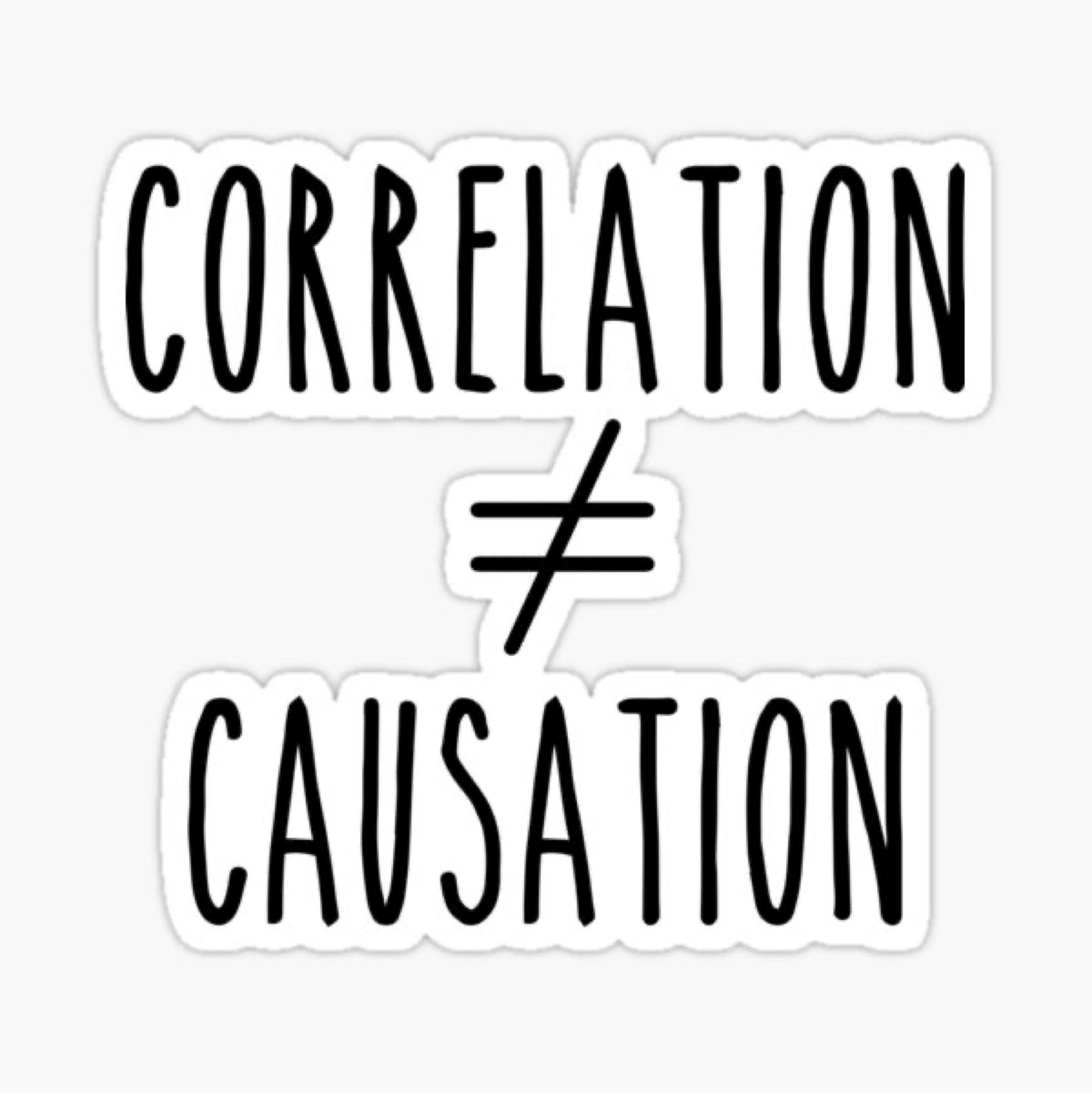
Correlation ≠ Causation
r
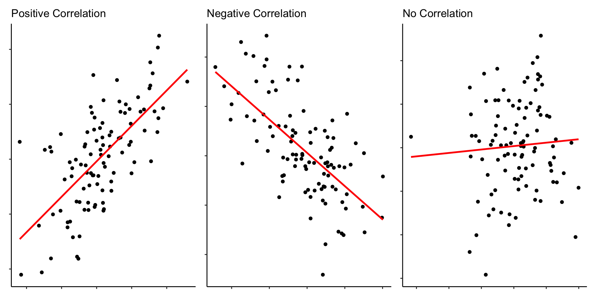
Positive correlation: variables move together
- As one goes up, the other goes up.
- As one goes down, the other goes down.

Correlation

Assesses how two variables move in relation to one another.

Ok, but how?!

Measures of Dispersion

What are measures of dispersion?
Measures of how spread out the data are, how much participants differ.

Measures of Dispersion

How do we measure dispersion when we were looking at one variable?
Standard deviation
Variance

Measures of Dispersion

Univariate = one variable
Bivariate = two variables
Multivariate = more than two variables

Measures of Dispersion

Univariate = one variable
Bivariate = two variables
Multivariate = more than two variables

Measures of Dispersion

Univariate measures of dispersion?
- Standard deviation: How different are participants from the average?
Bivariate measures of dispersion:
- Covariance
- How much variation in one variable is the same in another variable?
- Do the variables vary in the same way?

Measures of Dispersion

Univariate measures of dispersion?
Standard deviation: Height M = 5'6", s = 2 inches
Bivariate measures of dispersion:
- Covariance: Does the spread-out-ness of height overlap with the spread-out-ness of weight?

Covariance

Professor Brocker wants to know if how many cups of coffee a professor drinks daily impacts their happiness. She asks 50 professors how many cups they have in a typical day and then has them rate their happiness on a scale of 1 to 10.

Variable 1: Number of Cups of Coffee = continuous
Variable 2: Happiness = continuous

Covariance

We could:

Find the variance of each variable
Find the covariance of the two variables together

Covariance

Covariance refers to how two continuous variables vary in tandem.

Covariance

Covariance refers to how two variables vary together:

Generally, if cups of coffee goes up, what does happiness tend to do?
Generally, if happiness goes up, what does cups of coffee tend to do?

Covariance

Professor Brocker wants to know if how many cups of coffee a professor drinks daily impacts their happiness. She asks 50 professors how many cups they have in a typical day and then has them rate their happiness on a scale of 1 to 10.

Variable 1: Number of Cups of Coffee
Variable 2: Happiness

\[ COV_{XY} = \frac{\Sigma(X-\bar{X}(Y-\bar{Y})}{N-1} \]

Covariance

Well, well, well–We Meet Again

\[ COV_{XY} = \frac{\Sigma(X-\bar{X}(Y-\bar{Y})}{N-1} \]

\[ s^2 = \frac{\Sigma(X-\bar{X})^2}{N-1} \]

Covariance

\[ COV_{XY} = \frac{\Sigma(X-\bar{X}(Y-\bar{Y})}{N-1} \]

\[ s^2 = \frac{\Sigma(X-\bar{X})^2}{N-1} = \frac{\Sigma(X-\bar{X})(X-\bar{X})}{N-1} \]

Covariance

The variance of a variable is the covariance of that variable with itself.

\[ COV_{XY} = \frac{\Sigma(X-\bar{X}(Y-\bar{Y})}{N-1} \]

Covariance

Covariance is the variance of two variables together… how they move together.

\[ COV_{XY} = \frac{\Sigma(X-\bar{X})(Y-\bar{Y})}{N-1} \]

Covariance

Let’s break it down.

Find the mean of each variable.

\[\bar{X} = \frac{\Sigma(x)}{n}\] \[\bar{Y} = \frac{\Sigma(Y)}{n}\]

Covariance

Let’s break it down.

Find the mean of each variable.
Subtract the mean of x from each x value.
Subtract the mean of y from each y value.

\[(X-\bar{X})\] \[(Y-\bar{Y})\]

Covariance

Let’s break it down.

Find the mean of each variable.
Subtract the mean of x from each x value.
Subtract the mean of y from each y value.
Multiple the deviation scores of x with the deviation scores of y.

\[(X-\bar{X})(Y-\bar{Y})\]

Covariance

Let’s break it down.

Find the mean of each variable.
Subtract the mean of x from each x value.
Subtract the mean of y from each y value.
Multiple the deviation scores of x with the deviation scores of y.
Sum the products of the deviation scores.

\[\sum(X-\bar{X})(Y-\bar{Y})\]

Covariance

Let’s break it down.

Find the mean of each variable.
Subtract the mean of x from each x value.
Subtract the mean of y from each y value.
Multiple the deviation scores of x with the deviation scores of y.
Sum the products of the deviation scores.
Divide by N-1.

\[\frac{\sum(X-\bar{X})(Y-\bar{Y})}{N-1}\]

Covariance

Covariance is the bivariate equivalent of variance.

What does the covariance tell us?
What did the variance tell us?
- Not much because it was inflated.
For it to be useful, we had to standardize it.

\[ COV_{XY} = \frac{\Sigma(X-\bar{X})(Y-\bar{Y})}{N-1} \]

Correlation

Correlation is the standardized covariance.
Correlation is the bivariate version of the standard deviation.
To calculate the correlation, we divide the covariance by the standard deviation of x multipled by the standard deviation of y.

\[\frac{cov_{xy}}{(SD_x)(SD_y)}\]

Calculating Correlation:

Correlation

\[ COV_{XY} = \frac{\Sigma(X-\bar{X})(Y-\bar{Y})}{N-1} \] \[\frac{cov_{xy}}{(SD_x)(SD_y)}\]

Correlation

Calculating Correlation:

\[ \frac{\Sigma(X-\bar{X})(Y-\bar{Y})}{(SD_x)(SD_y)(N-1)} \]

Correlation

Correlation is the bivariate version of the standard deviation.

\[ \frac{\Sigma(X-\bar{X})(Y-\bar{Y})}{(SD_x)(SD_y)(N-1)} \]

Correlation

Correlation is bounded between -1 and +1.
Closer to -1 is a negative correlation.
Closer to +1 is a positive correlation.
Closer to 0 means no correlation.

Correlation

Correlation

This is the Pearson Product-Moment Correlation (Pearson, 1895).

The sign indicates the direction.
The number indicates the magnitude/strength of the relationship.
- 0.1 is a small correlation
- 0.3 is a moderate correlation
- 0.5 or higher is a large correlation

Correlation

Correlation is written as r
If we square r, we get \(R^2\)
\(R^2\) is always positive
\(R^2\) refers to:
- The amount of x accounted for by y.
- The amount of y accounted for by x.

Correlation and \(R^2\)

Example

Students grades in MTH 110 and their grades in correlation at r = 0.3

Moderate correlation
How much of your grade is accounted for by your MTH 110 grade?
0.3 x 0.3 = 0.09
\(R^2\) = 9% of your grade is explained by your MTH 110 grade.

Interpreting Correlation

We don’t use the words caused/resulting from.
When reporting r: “As x goes up, y tends to go up.”
When reporting \(R^2\): “z% of x is accounted for by y.”

Reporting correlation

Correlation Matrix

In the Method, we report descriptive statistics about our variables (M, s).
It is common to refer readers to a table where they can look at correlations between the variables.
Why might this be important?

Correlation Matrix

Table 1 in a paper is typically a combination of descriptive stats AND correlation matrix, like this:

	M	s	1	2	3
Age	20.9	1.76	1	--	--
Song 1	4.21	1.2	.03	1	--
Song 2	6.42	2.18	.65**	-.34*	1

Correlation Matrix

Table 1 in a paper is typically a combination of descriptive stats AND correlation matrix, like this:

	M	s	1	2	3
Age	20.9	1.76	1	-.03	.65**
Song 1	4.21	1.2	-.03	1	-.34*
Song 2	6.42	2.18	.65**	-.34*	1

Reporting Calculation

Example 1

In a psychology experiment, researchers collected data on the number of hours spent studying and the scores on a final exam for 50 students. Below is a scatterplot showing the relationship between the two variables.

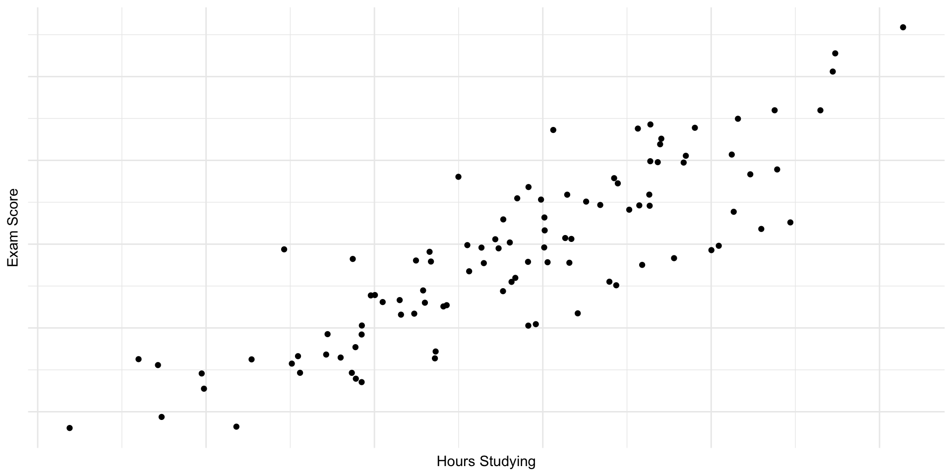
Based on the scatterplot, describe the strength and direction of the relationship between hours spent studying and exam scores. Would you say the correlation is weak, moderate, or strong? Is it positive or negative?

Reporting Calculation

Example 1

Suppose the computed Pearson correlation coefficient is r = 0.85 . Explain what this value indicates about the relationship between the two variables.

Reporting Calculation

Example 2

Using the same data from the previous question, the researchers fit a linear regression model to predict exam scores from the number of hours spent studying. The \(R^2\) value for the model is 0.72.

What does an \(R^2\) value of 0.72 tell you about how well hours spent studying explain the variance in exam scores? What percentage of the variance is explained by the model, and what percentage remains unexplained?
Imagine you are the researcher. Based on the \(R^2\) value of 0.72, would you consider study time to be a good predictor of exam performance? Why or why not?