   student before after
1        1     21    20
2        2     17    13
3        3     23    19
4        4     27    24
5        5     20    21
6        6     21    15
7        7     15    11
8        8     23    26
9        9     20    18
10      10     16     9
11      11     27    29
12 12 15 9Lab 6: The Paired-Samples t-Test
Testing Whether the Same People Changed Between Two Measurements
Dave Brocker
Farmingdale State College
Quick Recap
\[t = \frac{\bar{x} - \mu}{s / \sqrt{n}} \qquad\qquad t = \frac{\bar{D}}{s_D / \sqrt{n}}\]
Last lab: a one-sample t-test compared one sample mean to a known value
Today: the same people are measured twice (before and after, or under two conditions)
A paired-samples t-test is a one-sample t-test on the difference scores: is the mean difference \(\bar{D}\) different from 0?
Same habit as before: write every argument by name
Where \(\bar{D}\) and \(s_D\) Come From
\[D_i = x_{i,\text{after}} - x_{i,\text{before}} \qquad \bar{D} = \frac{\sum D_i}{n} \qquad s_D = \sqrt{\frac{\sum (D_i - \bar{D})^2}{n - 1}}\]
\(D_i\) is each person’s own change (after minus before)
\(\bar{D}\) is the average change; \(s_D\) is how much the changes vary from person to person
\(\dfrac{s_D}{\sqrt{n}}\) is the estimated standard error of the mean difference, and \(df = n - 1\) counts pairs
Scenario
12PSY 348 students rated their anxiety (0 to 30) right before a quiz. They then did a 5-minute breathing exercise and rated their anxiety again.
\(H_0: \mu_D = 0\) (the exercise does not change anxiety)
\(H_A: \mu_D \neq 0\) (anxiety changes: a two-tailed test)
\(\alpha = .05\)
Each student has two scores, so this is a paired-samples t-test
Our Data
anxiety_data.R
Step 1: Difference Scores
By Hand First
\[t = \frac{\bar{D}}{s_D/\sqrt{n}} = \frac{-2.58}{3.26/\sqrt{12}} = \frac{-2.58}{0.94} = -2.74\]
\(df = n - 1 = 12 - 1 = 11\)
The two-tailed critical value for \(df = 11\) is \(\pm 2.20\)
\(|-2.74| > 2.20\), so we expect to reject \(H_0\)
Now in R: Step by Step
paired_by_hand.R
n      <- length(x = D)
d_bar  <- mean(x = D)
s_d    <- sd(x = D)

se     <- s_d / sqrt(x = n)                # estimated standard error
t      <- d_bar / se                       # compared with 0, so nothing to subtract
df     <- n - 1

# Two-tailed p: area beyond |t| in one tail, doubled
p      <- 2 * pt(q = abs(x = t), df = df, lower.tail = FALSE)

# Critical value: the t that leaves 2.5% in each tail
t_crit <- qt(p = 0.975, df = df, lower.tail = TRUE)

c(se = se, t = t, df = df, p = p, t_crit = t_crit)
se t df p t_crit
0.94113353 -2.74491690 11.00000000 0.01906313 2.20098516 One Function: t.test()
paired_t_test.R
    Paired t-test

data:  after and before
t = -2.7449, df = 11, p-value = 0.01906
alternative hypothesis: true mean difference is not equal to 0
95 percent confidence interval:
 -4.6547543 -0.5119124
sample estimates:
mean difference
      -2.583333
Same t, df, and p as our step-by-step version.
x - yis after minus before: the order sets the signThe interval (about -4.65 to -0.51) is for the mean difference and excludes
0paired = TRUEtells R the two columns are the same people
Paired Is a One-Sample Test on \(D\)
one_sample_on_d.R
Identical t, df, p, and interval: the pairing only matters for making the difference scores
After that, it is Lab 5 again, with \(\mu_0 = 0\)
Why Pairing Helps
paired_vs_independent.R
Students differ a lot from each other (some start at 15, some at 27). The independent test treats that as noise
Pairing compares each person with themselves, so the between-person differences drop out and the real change shows
Seeing the Test
Click Code to see how the plot is built.
Code
library(ggplot2)

long <- data.frame(
  student = rep(x = 1:12, times = 2),
  time    = factor(x = rep(x = c("Before", "After"), each = 12), levels = c("Before", "After")),
  anxiety = c(before, after)
)

ggplot(data = long, mapping = aes(x = time, y = anxiety, group = student)) +
  geom_line(color = "grey60") +
  geom_point(size = 3) +
  stat_summary(mapping = aes(group = 1), fun = mean, geom = "line",
               color = "orange", linewidth = 1.8) +
  theme_minimal(base_size = 18) +
  labs(
    title = "Each Grey Line Is One Student; Orange Is the Group Mean",
    x = NULL, y = "Anxiety (0 to 30)"
  ) +
  theme(panel.grid.minor = element_blank())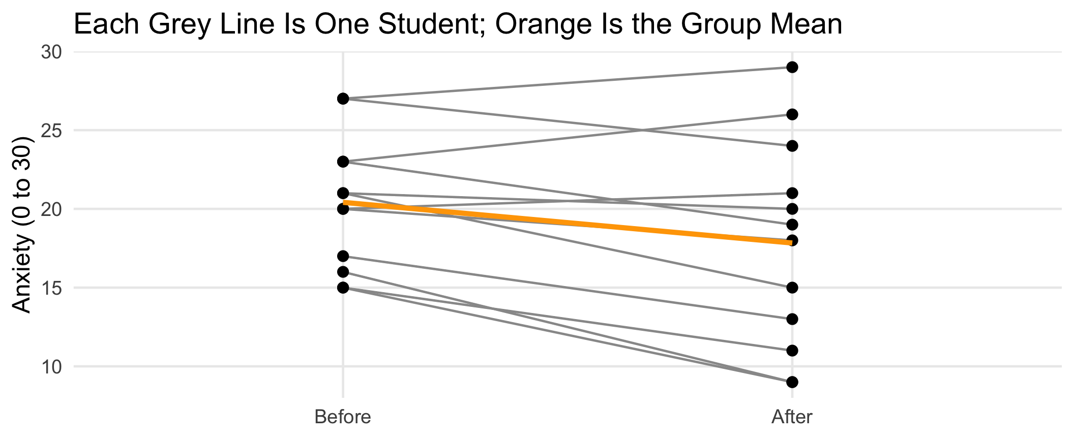
Effect Size and APA Write-Up
\[d_z = \frac{\bar{D}}{s_D} = \frac{-2.58}{3.26} = -0.79\]
Anxiety decreased after the breathing exercise, M_D = -2.58, SD_D = 3.26, t(11) = -2.74, p = .019, d_z = -0.79.
The negative sign only says anxiety went down. \(|d_z| = 0.79\) sits right at the medium/large boundary (0.8): a substantial effect
Your Turn
The Data
Does a phone in the room cost you memory? 10 students studied word lists in two sessions, once with their phone near them and once with it away in a bag. We expect they recall more words with the phone away.
recall_data.R
   student near away
1        1   14   19
2        2   15   19
3        3   12   11
4        4   15   18
5        5   18   18
6        6   14   18
7        7   17   18
8        8   14   17
9        9   13   12
10      10   10   11
Questions 1 to 3
Write every argument by name. Use \(\alpha = .05\) and define \(D = \text{away} - \text{near}\).
State \(H_0\) and \(H_A\) in terms of \(\mu_D\). Then compute the difference scores \(D\) and find \(\bar{D}\), \(s_D\), the standard error, and \(t\) by hand (use R only for
mean()andsd()).What are the degrees of freedom? Use
qt()to find the two-tailed critical value, and the one-tailed critical value for \(H_A: \mu_D > 0\).Run
t.test()withpaired = TRUEand a two-tailed alternative. Report t, df, p, and the 95% confidence interval. Do you reject \(H_0\)?
Questions 4 to 6
Now run
t.test()withalternative = "greater". How does the p-value change, and does your decision change? (Check which directionx - ypoints first.)Run the test again ignoring the pairing (
paired = FALSE, var.equal = TRUE). Compare the p-values. Why does pairing help here?Compute \(d_z = \dfrac{\bar{D}}{s_D}\) and write an APA-style sentence for the one-tailed test.
Submit on Brightspace
Your answers to the six questions above (show your R code and output)
One sentence: why is a paired-samples t-test the same as a one-sample t-test?
PSY 348 - Statistics for Psychology