Lab 5: The One-Sample t-Test

Testing a Sample Mean When σ Is Unknown

Dave Brocker

Farmingdale State College

Quick Recap

\[z = \frac{\bar{x} - \mu}{\sigma / \sqrt{n}} \qquad\qquad t = \frac{\bar{x} - \mu}{s / \sqrt{n}}\]

• Last lab we knew the population standard deviation \(\sigma\), so we used z

• Usually we do not know \(\sigma\), so we estimate it with the sample standard deviation \(s\) and use t

• The t distribution has fatter tails than z, and it depends on the degrees of freedom: \(df = n - 1\)

• Same habit as before: write every argument by name

Where Does \(s\) Come From?

\[s = \sqrt{\frac{\sum (x - \bar{x})^2}{n - 1}}\]

• Numerator: every score’s squared distance from the mean, added up

• Denominator: \(n - 1\), and then we take the square root

• \(\dfrac{s}{\sqrt{n}}\) is the estimated standard error: how much sample means bounce around

Scenario

A national survey says college students spend 9 hours a week studying outside of class. We asked 12 PSY 348 students how many hours they studied last week.

• \(H_0: \mu = 9\) (our students study the same as the national average)

• \(H_A: \mu \neq 9\) (they study a different amount: a two-tailed test)

• \(\alpha = .05\)

• We do not know \(\sigma\), so this is a one-sample t-test

Our Data

study_data.R

set.seed(seed = 348)
study_hours <- round(x = rnorm(n = 12, mean = 12, sd = 4), digits = 0)

study_hours

 [1] 12 16 15  4  9 15  9  9 14 21 10 18

c(n = length(x = study_hours),
  mean = mean(x = study_hours),
  sd = sd(x = study_hours))

        n      mean        sd 
12.000000 12.666667  4.716187 

By Hand First

\[t = \frac{\bar{x} - \mu}{s/\sqrt{n}} = \frac{12.67 - 9}{4.72/\sqrt{12}} = \frac{3.67}{1.36} = 2.69\]

• \(df = n - 1 = 12 - 1 = 11\)

• The two-tailed critical value for \(df = 11\) is \(\pm 2.20\)

• \(|2.69| > 2.20\), so we expect to reject \(H_0\)

Now in R: Step by Step

t_by_hand.R

mu_0 <- 9                                  # the value in H0
n    <- length(x = study_hours)
m    <- mean(x = study_hours)
s    <- sd(x = study_hours)

se   <- s / sqrt(x = n)                    # estimated standard error
t    <- (m - mu_0) / se
df   <- n - 1

# Two-tailed p: area beyond |t| in one tail, doubled
p    <- 2 * pt(q = abs(x = t), df = df, lower.tail = FALSE)

# Critical value: the t that leaves 2.5% in each tail
t_crit <- qt(p = 0.975, df = df, lower.tail = TRUE)

c(se = se, t = t, df = df, p = p, t_crit = t_crit)

         se           t          df           p      t_crit 
 1.36144605  2.69321481 11.00000000  0.02090871  2.20098516 

One Function: t.test()

t_test.R

t.test(x = study_hours, mu = 9, alternative = "two.sided", conf.level = 0.95)

    One Sample t-test

data:  study_hours
t = 2.6932, df = 11, p-value = 0.02091
alternative hypothesis: true mean is not equal to 9
95 percent confidence interval:
  9.670144 15.663189
sample estimates:
mean of x 
 12.66667 

• Same t, df, and p as our step-by-step version

• alternative can be "two.sided", "less", or "greater"

• The confidence interval (about 9.67 to 15.66) does not contain 9: another way to see the rejection

Seeing the Test

Click Code to see how the plot is built.

library(ggplot2)

curve_df <- data.frame(x = seq(from = -4, to = 4, by = 0.01))
curve_df$y <- dt(x = curve_df$x, df = 11)

ggplot(data = curve_df, mapping = aes(x = x, y = y)) +
  geom_line(linewidth = 1.1) +
  geom_area(data = subset(x = curve_df, subset = x >= abs(x = t)), fill = "orange", alpha = 0.6) +
  geom_area(data = subset(x = curve_df, subset = x <= -abs(x = t)), fill = "orange", alpha = 0.6) +
  geom_vline(xintercept = c(-t_crit, t_crit), linetype = "dashed") +
  theme_minimal(base_size = 18) +
  labs(
    title = "t Distribution (df = 11): Shaded Area Is the Two-Tailed p-Value",
    x = "\nt", y = "Density\n"
  ) +
  theme(panel.grid = element_blank())

Effect Size and APA Write-Up

\[d = \frac{\bar{x} - \mu}{s} = \frac{12.67 - 9}{4.72} = 0.78\]

cohens_d.R

d <- (m - mu_0) / s
round(x = d, digits = 2)

[1] 0.78

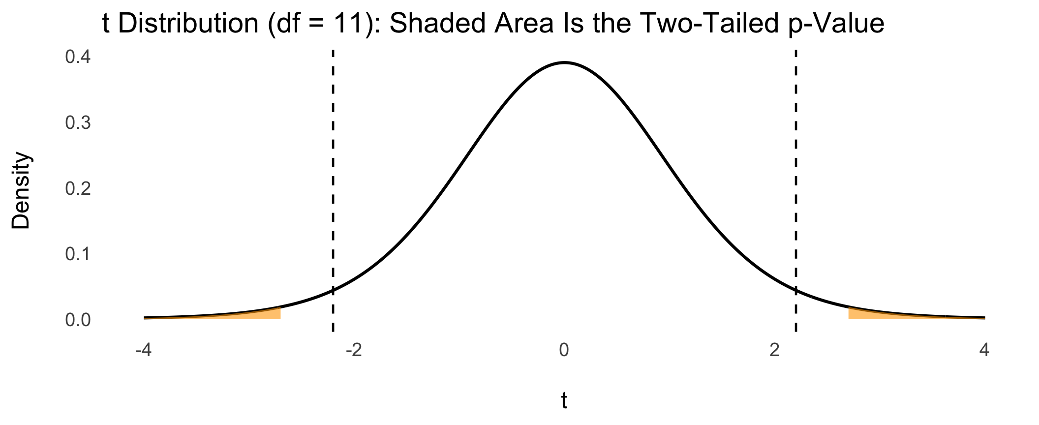
• Students studied more than the national average of 9 hours, M = 12.67, SD = 4.72, t(11) = 2.69, p = .021, d = 0.78.

• By the usual benchmarks, \(d \approx 0.8\) is a large effect

Your Turn

The Data

Sleep researchers recommend at least 7 hours a night. We asked 10 students how many hours they slept last night, and we expect they sleep less than 7.

sleep_data.R

set.seed(seed = 133)
sleep_hours <- round(x = rnorm(n = 10, mean = 6.5, sd = 0.9), digits = 1)

sleep_hours

 [1] 6.6 6.8 5.8 6.8 7.6 6.5 7.4 6.4 6.3 5.3

Questions 1 to 3

Write every argument by name. Use \(\mu = 7\) and \(\alpha = .05\).

1. By hand (use R only for mean() and sd()): find \(\bar{x}\), \(s\), the standard error, and \(t\).

2. What are the degrees of freedom? Use qt() to find the two-tailed critical value, and the one-tailed critical value for \(H_A: \mu < 7\).

3. Run t.test() with a two-tailed alternative. Report t, df, p, and the 95% confidence interval. Do you reject \(H_0\)?

Questions 4 and 5

4. Now run t.test() with alternative = "less". How does the p-value change, and does your decision change? Why must you choose one-tailed or two-tailed before looking at the data?

5. Write an APA-style sentence reporting the result of the one-tailed test, and compute Cohen’s \(d = \dfrac{\bar{x} - \mu}{s}\). Is the effect small, medium, or large?

Submit on Brightspace

• Your answers to the five questions above (show your R code and output)

• One sentence: why do we use \(t\) instead of \(z\) when we do not know \(\sigma\)?