Lab 4: Z-Scores, Sampling & the Z-Test

Standardizing Data, Finding Probabilities, and Testing a Sample Mean

Dave Brocker

Farmingdale State College

Quick Recap

\[z = \frac{x - \mu}{\sigma}\]

  • A z-score tells you how many standard deviations a value is from the mean

  • Once we have a z-score, we can find probabilities: what proportion of scores fall above, below, or between values

  • Today’s habit: we will write out every argument by name (mean =, sd =, lower.tail =). It is more typing, but you never have to guess what a number is doing.

Part 1: Z-Scores and Probability

Scenario

Professor Brocker’s PSY 348 midterm had 40 students. The exam scores were approximately normally distributed with a mean of 76 and a standard deviation of 8.

  • Nadia scored an 88.

  • Before we calculate anything: is that a good score relative to the class? Great? Just okay?

By Hand First

\[z = \frac{x - \mu}{\sigma} = \frac{88 - 76}{8} = 1.5\]

  • Nadia’s score is 1.5 standard deviations above the mean

  • Using the 68/95/99.7 rule: roughly 93% of students scored below Nadia

Now in R: One Score

We store the facts first, so every later line says what each number is.

z_one_score.R

mu    <- 76    # population mean of the exam
sigma <- 8     # population standard deviation
nadia <- 88    # Nadia's raw score

z_nadia <- (nadia - mu) / sigma
z_nadia
[1] 1.5

Two Roads to the Same Probability

pnorm() returns the probability of scoring at or below a value: \(P(X \le x) = P\!\left(Z \le \dfrac{x - \mu}{\sigma}\right)\), the area to the left of the z-score.

pnorm_two_ways.R

# Road 1: give pnorm() the RAW score, plus the mean and sd
pnorm(q = 88, mean = 76, sd = 8, lower.tail = TRUE)
[1] 0.9331928
# Road 2: standardize first, then use the STANDARD normal
pnorm(q = 1.5, mean = 0, sd = 1, lower.tail = TRUE)
[1] 0.9331928
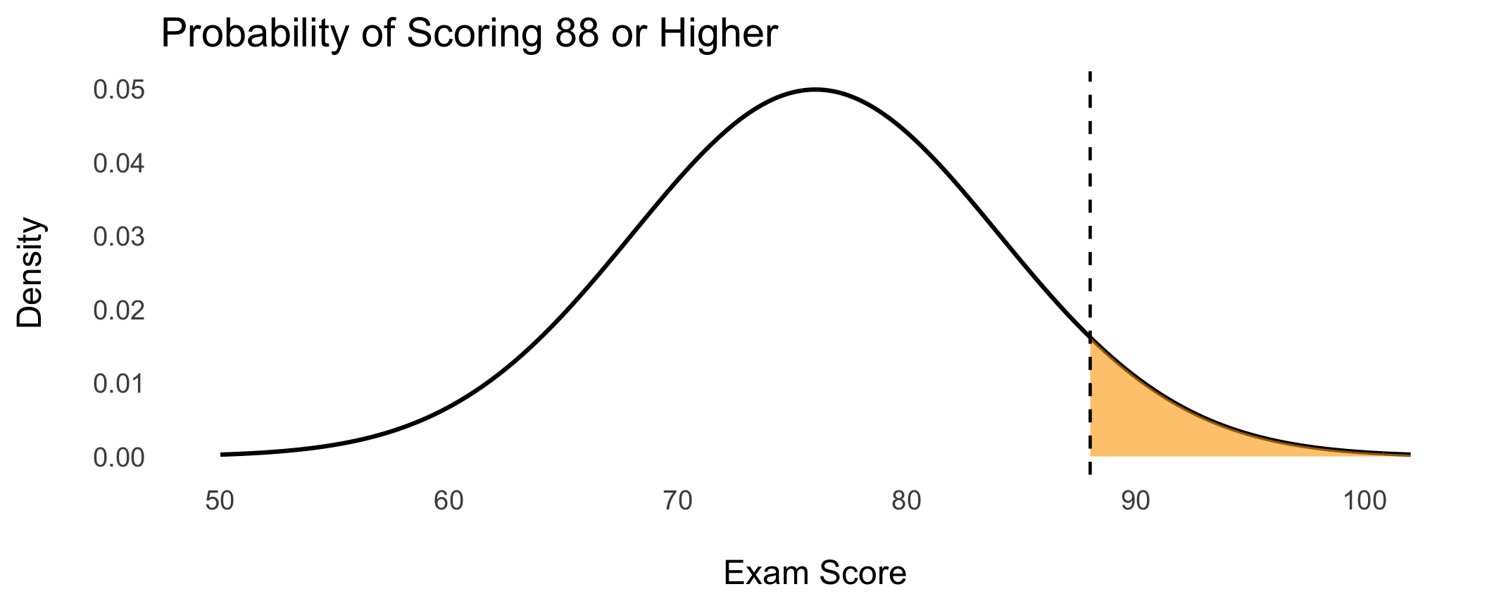
  • Same answer: 93.3% score at or below Nadia, so about 6.7% outscore her

  • Raw score + the real mean and sd = z-score + mean = 0, sd = 1

  • Mixing them (a raw score with mean = 0, sd = 1) is the most common mistake in this lab

Visualizing It

Click Code to see how the plot is built.

Code
library(ggplot2)

dat <- data.frame(x = seq(from = 50, to = 102, by = 0.1))
dat$y <- dnorm(x = dat$x, mean = 76, sd = 8)

ggplot(data = dat, mapping = aes(x = x, y = y)) +
  geom_line(linewidth = 1.1) +
  geom_area(
    data = subset(dat, x >= 88),
    fill = "orange", alpha = 0.6
  ) +
  geom_vline(xintercept = 88, linetype = "dashed") +
  theme_minimal(base_size = 18) +
  labs(
    title = "Probability of Scoring 88 or Higher",
    x = "\nExam Score",
    y = "Density\n"
  ) +
  theme(panel.grid = element_blank())
Going the Other Direction

qnorm() does the reverse: give it a probability, get back a score.

qnorm_top10.R

# What score marks the top 10% of the class?
# Top 10% means 90% are at or below it.
qnorm(p = 0.90, mean = 76, sd = 8, lower.tail = TRUE)
[1] 86.25241
  • A student would need roughly an 86 to be in the top 10% of this class

Standardizing a Whole Class

Now we simulate 40 students. scale() converts every score to a z-score at once.

scale_class.R

set.seed(seed = 348)
exam_scores <- round(rnorm(n = 40, mean = 76, sd = 8), digits = 1)

z_scores <- round(scale(x = exam_scores, center = TRUE, scale = TRUE)[, 1], digits = 2)

head(data.frame(score = exam_scores, z = z_scores), n = 8)
  score     z
1  76.6  0.14
2  83.9  1.09
3  82.3  0.88
4  59.2 -2.11
5  69.8 -0.74
6  82.6  0.92
7  70.8 -0.61
8  69.5 -0.78
  • What do you notice about the mean of z_scores? The standard deviation?

What mean() and sd() Compute

\[\bar{x} = \frac{\sum x}{n} \qquad s = \sqrt{\frac{\sum (x - \bar{x})^2}{n - 1}}\]

The numerator of \(s\) adds up each score’s squared distance from the mean. Dividing by \(n - 1\) and taking the square root gives the typical distance of a score from the mean.

Population vs. This Class

Our 40 simulated scores are a sample, so their mean and sd are close to, but not exactly, 76 and 8.

class_vs_population.R

mean(x = exam_scores)   # this class
[1] 75.4875
sd(x = exam_scores)     # this class
[1] 7.70222
(88 - mean(x = exam_scores)) / sd(x = exam_scores)   # Nadia vs. THIS class
[1] 1.624532
(88 - 76) / 8                                        # Nadia vs. the POPULATION
[1] 1.5
  • The two z-scores differ slightly. Neither is wrong: they answer different questions (how does she compare to these 40 vs. to every possible student)

Part 2: Sampling and the Z-Test

From One Score to a Sample Mean

Nadia is one student. What if we care about the average of a whole class?

  • A single score varies a lot from student to student

  • An average of many scores varies much less

  • So a sample mean needs a different yardstick than a single score

Simulating a Sampling Distribution

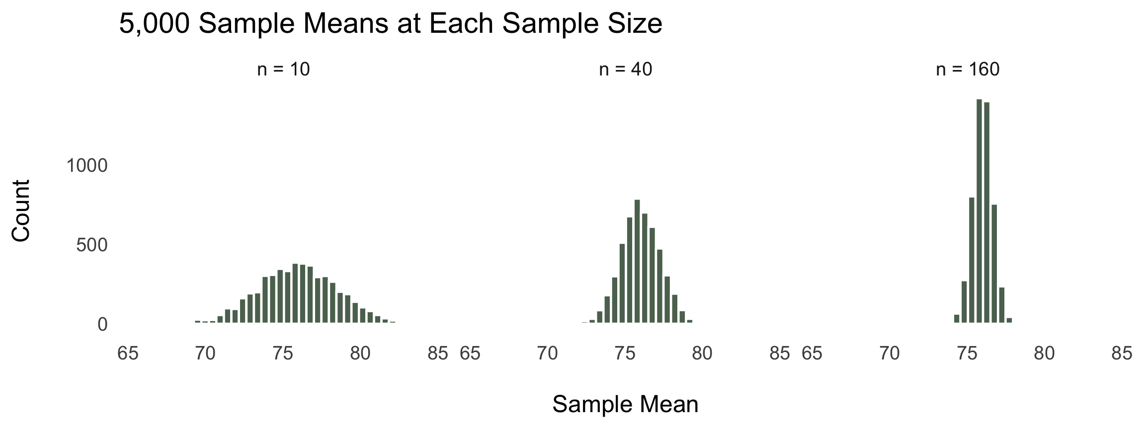
Draw many samples of size n, record each sample’s mean, then look at how those means are spread out. The sd() of these simulated means is the standard error, \(SE = \dfrac{\sigma}{\sqrt{n}}\) (next slides).

sampling_sim.R

set.seed(seed = 348)

sim_means <- function(n) {
  replicate(n = 5000, expr = mean(x = rnorm(n = n, mean = 76, sd = 8)))
}

means_10  <- sim_means(n = 10)
means_40  <- sim_means(n = 40)
means_160 <- sim_means(n = 160)

sd(x = means_10)    # spread of the sample means when n = 10
[1] 2.571714
sd(x = means_40)    # n = 40
[1] 1.273569
sd(x = means_160)   # n = 160
[1] 0.6340208

Bigger Samples, Narrower Distribution

Code
library(dplyr)

sims <- bind_rows(
  data.frame(mean = means_10,  n = "n = 10"),
  data.frame(mean = means_40,  n = "n = 40"),
  data.frame(mean = means_160, n = "n = 160")
) |>
  mutate(n = factor(x = n, levels = c("n = 10", "n = 40", "n = 160")))

ggplot(data = sims, mapping = aes(x = mean)) +
  geom_histogram(bins = 40, fill = "#5C715E", color = "white") +
  facet_wrap(facets = ~ n) +
  theme_minimal(base_size = 18) +
  labs(
    title = "5,000 Sample Means at Each Sample Size",
    x = "\nSample Mean", y = "Count\n"
  ) +
  theme(panel.grid = element_blank())
Standard Error

The spread of the sample means has a name: the standard error.

\[SE = \frac{\sigma}{\sqrt{n}}\]

standard_error.R

sigma <- 8

sigma / sqrt(x = 10)    # n = 10
[1] 2.529822
sigma / sqrt(x = 40)    # n = 40
[1] 1.264911
sigma / sqrt(x = 160)   # n = 160
[1] 0.6324555
  • Compare to the simulated spreads on the previous slide: they match
  • Quadruple n and the standard error is cut in half

Individual z vs. Sample-Mean z

Same population: \(\mu = 76\), \(\sigma = 8\).

Question Formula Result
Nadia scored 88. How unusual is she? \(z = \dfrac{88 - 76}{8}\) \(z = 1.5\)
A class of 40 averaged 80. How unusual is that class? \(z = \dfrac{80 - 76}{8/\sqrt{40}}\) \(z \approx 3.16\)
  • A score of 88 is uncommon. A class mean of 80 is far rarer, because means vary much less than single scores
  • The only change in the formula: divide by the standard error, not by \(\sigma\)

Setting Up the Z-Test

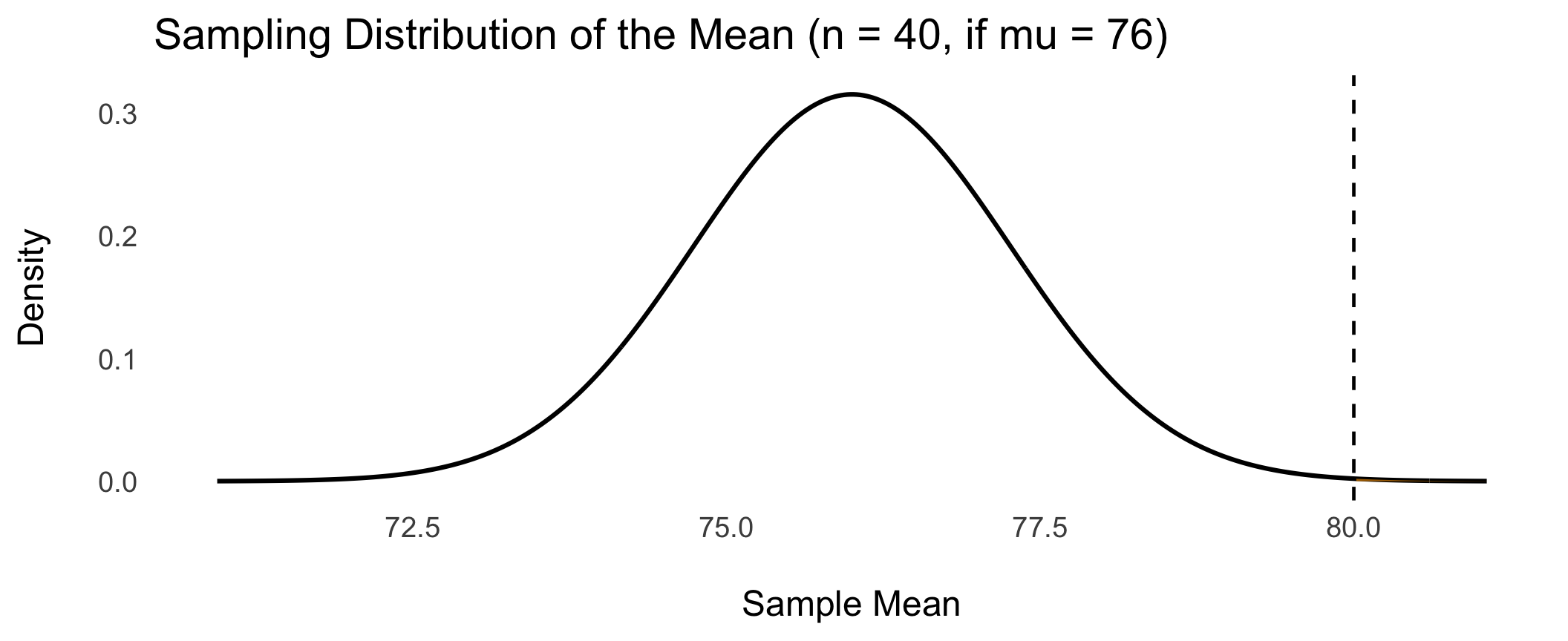
Question: a class of n = 40 averaged 80. If the population mean really is 76 (with \(\sigma = 8\)), how likely is a class mean this high?

\[z = \frac{\bar{x} - \mu}{\sigma / \sqrt{n}}\]

The numerator is how far the sample mean sits from the population mean. The denominator is the standard error, so z counts standard errors.

The One-Sample Z-Test in R

z_test.R

mu     <- 76    # population mean
sigma  <- 8     # population standard deviation
n      <- 40    # sample size
m      <- 80    # observed sample mean

se <- sigma / sqrt(x = n)
z  <- (m - mu) / se

# One-tailed: P(sample mean >= 80)
p_one <- pnorm(q = z, mean = 0, sd = 1, lower.tail = FALSE)

# Two-tailed: the extreme could have been in either direction
p_two <- 2 * p_one

c(se = se, z = z, p_one = p_one, p_two = p_two)
          se            z        p_one        p_two 
1.2649110641 3.1622776602 0.0007827011 0.0015654023 
  • The p-value is tiny (far below .05): a mean of 80 would be very surprising if \(\mu\) were really 76
  • Note lower.tail = FALSE: we want the area above z

Seeing the Test

Code
se <- 8 / sqrt(x = 40)

dat2 <- data.frame(x = seq(from = 76 - 4 * se, to = 76 + 4 * se, length.out = 400))
dat2$y <- dnorm(x = dat2$x, mean = 76, sd = se)

ggplot(data = dat2, mapping = aes(x = x, y = y)) +
  geom_line(linewidth = 1.1) +
  geom_area(data = subset(dat2, x >= 80), fill = "orange", alpha = 0.6) +
  geom_vline(xintercept = 80, linetype = "dashed") +
  theme_minimal(base_size = 18) +
  labs(
    title = "Sampling Distribution of the Mean (n = 40, if mu = 76)",
    x = "\nSample Mean", y = "Density\n"
  ) +
  theme(panel.grid = element_blank())
Your Turn

Use the exam setting: \(\mu = 76\), \(\sigma = 8\). Write every argument by name.

  1. Calculate the z-score for a student who scored a 70. Is that above or below average?

  2. Using pnorm(), what proportion of the population scored below a 70?

  3. Using qnorm(), what raw score marks the bottom 25%?

Your Turn (continued)

Same setting: \(\mu = 76\), \(\sigma = 8\).

  1. What is the standard error when n = 25? When n = 100? By what factor did it shrink?

  2. A different class of n = 25 averaged 79. Run a two-tailed z-test against \(\mu = 76\). Report the standard error, z, and p-value.

  3. In your own words: why can a class mean of 79 be “unusual” when an individual score of 79 is not?

Submit on Brightspace

  • Your answers to the six questions above (show your R code and output)

  • One sentence: is a z-score of 0 a “good” or “bad” score? Explain.